The system of linear equations is called joint if mti. Solving systems of linear equations using the Jordan-Gauss method

Lesson content

Linear Equations with Two Variables

The student has 200 rubles to have lunch at school. A cake costs 25 rubles, and a cup of coffee costs 10 rubles. How many cakes and cups of coffee can you buy for 200 rubles?

Denote the number of cakes through x, and the number of cups of coffee through y. Then the cost of cakes will be denoted by the expression 25 x, and the cost of cups of coffee in 10 y .

25x- price x cakes
10y- price y cups of coffee

The total amount should be 200 rubles. Then we get an equation with two variables x and y

25x+ 10y= 200

How many roots does this equation have?

It all depends on the appetite of the student. If he buys 6 cakes and 5 cups of coffee, then the roots of the equation will be the numbers 6 and 5.

The pair of values 6 and 5 are said to be the roots of Equation 25 x+ 10y= 200 . Written as (6; 5) , with the first number being the value of the variable x, and the second - the value of the variable y .

6 and 5 are not the only roots that reverse Equation 25 x+ 10y= 200 to identity. If desired, for the same 200 rubles, a student can buy 4 cakes and 10 cups of coffee:

In this case, the roots of equation 25 x+ 10y= 200 is the pair of values (4; 10) .

Moreover, a student may not buy coffee at all, but buy cakes for all 200 rubles. Then the roots of equation 25 x+ 10y= 200 will be the values 8 and 0

Or vice versa, do not buy cakes, but buy coffee for all 200 rubles. Then the roots of equation 25 x+ 10y= 200 will be the values 0 and 20

Let's try to list all possible roots of equation 25 x+ 10y= 200 . Let us agree that the values x and y belong to the set of integers. And let these values be greater than or equal to zero:

x∈Z, y∈ Z;
x ≥ 0, y ≥ 0

So it will be convenient for the student himself. Cakes are more convenient to buy whole than, for example, several whole cakes and half a cake. Coffee is also more convenient to take in whole cups than, for example, several whole cups and half a cup.

Note that for odd x it is impossible to achieve equality under any y. Then the values x there will be the following numbers 0, 2, 4, 6, 8. And knowing x can be easily determined y

Thus, we got the following pairs of values (0; 20), (2; 15), (4; 10), (6; 5), (8; 0). These pairs are solutions or roots of Equation 25 x+ 10y= 200. They turn this equation into an identity.

Type equation ax + by = c called linear equation with two variables. A solution or roots of this equation is a pair of values ( x; y), which turns it into an identity.

Note also that if a linear equation with two variables is written as ax + b y = c , then they say that it is written in canonical(normal) form.

Some linear equations in two variables can be reduced to canonical form.

For example, the equation 2(16x+ 3y- 4) = 2(12 + 8x − y) can be brought to mind ax + by = c. Let's open the brackets in both parts of this equation, we get 32x + 6y − 8 = 24 + 16x − 2y . The terms containing unknowns are grouped on the left side of the equation, and the terms free of unknowns are grouped on the right. Then we get 32x - 16x+ 6y+ 2y = 24 + 8 . We bring similar terms in both parts, we get equation 16 x+ 8y= 32. This equation is reduced to the form ax + by = c and is canonical.

Equation 25 considered earlier x+ 10y= 200 is also a two-variable linear equation in canonical form. In this equation, the parameters a , b and c are equal to the values 25, 10 and 200, respectively.

Actually the equation ax + by = c has an infinite number of solutions. Solving the Equation 25x+ 10y= 200, we looked for its roots only on the set of integers. As a result, we obtained several pairs of values that turned this equation into an identity. But on the set rational numbers equation 25 x+ 10y= 200 will have an infinite number of solutions.

To get new pairs of values, you need to take an arbitrary value for x, then express y. For example, let's take a variable x value 7. Then we get an equation with one variable 25×7 + 10y= 200 in which to express y

Let x= 15 . Then the equation 25x+ 10y= 200 becomes 25 × 15 + 10y= 200. From here we find that y = −17,5

Let x= −3 . Then the equation 25x+ 10y= 200 becomes 25 × (−3) + 10y= 200. From here we find that y = −27,5

System of two linear equations with two variables

For the equation ax + by = c you can take any number of times arbitrary values for x and find values for y. Taken separately, such an equation will have an infinite number of solutions.

But it also happens that the variables x and y connected not by one, but by two equations. In this case, they form the so-called system linear equations with two variables. Such a system of equations can have one pair of values (or in other words: “one solution”).

It may also happen that the system has no solutions at all. A system of linear equations can have an infinite number of solutions in rare and exceptional cases.

Two linear equations form a system when the values x and y are included in each of these equations.

Let's go back to the very first equation 25 x+ 10y= 200 . One of the pairs of values for this equation was the pair (6; 5) . This is the case when 200 rubles could buy 6 cakes and 5 cups of coffee.

We compose the problem so that the pair (6; 5) becomes the only solution for equation 25 x+ 10y= 200 . To do this, we compose another equation that would connect the same x cakes and y cups of coffee.

Let's put the text of the task as follows:

“A schoolboy bought several cakes and several cups of coffee for 200 rubles. A cake costs 25 rubles, and a cup of coffee costs 10 rubles. How many cakes and cups of coffee did the student buy if it is known that the number of cakes is one more than the number of cups of coffee?

We already have the first equation. This is Equation 25 x+ 10y= 200 . Now let's write an equation for the condition "the number of cakes is one unit more than the number of cups of coffee" .

The number of cakes is x, and the number of cups of coffee is y. You can write this phrase using the equation x − y= 1. This equation would mean that the difference between cakes and coffee is 1.

x=y+ 1 . This equation means that the number of cakes is one more than the number of cups of coffee. Therefore, to obtain equality, one is added to the number of cups of coffee. This can be easily understood if we use the weight model that we considered when studying the simplest problems:

Got two equations: 25 x+ 10y= 200 and x=y+ 1. Since the values x and y, namely 6 and 5 are included in each of these equations, then together they form a system. Let's write down this system. If the equations form a system, then they are framed by the sign of the system. The system sign is a curly brace:

Let's solve this system. This will allow us to see how we arrive at the values 6 and 5. There are many methods for solving such systems. Consider the most popular of them.

Substitution method

The name of this method speaks for itself. Its essence is to substitute one equation into another, having previously expressed one of the variables.

In our system, nothing needs to be expressed. In the second equation x = y+ 1 variable x already expressed. This variable is equal to the expression y+ 1 . Then you can substitute this expression in the first equation instead of the variable x

After substituting the expression y+ 1 into the first equation instead x, we get the equation 25(y+ 1) + 10y= 200 . This is a linear equation with one variable. This equation is quite easy to solve:

We found the value of the variable y. Now we substitute this value into one of the equations and find the value x. For this, it is convenient to use the second equation x = y+ 1 . Let's put the value into it y

So the pair (6; 5) is a solution to the system of equations, as we intended. We check and make sure that the pair (6; 5) satisfies the system:

Example 2

Substitute the first equation x= 2 + y into the second equation 3 x - 2y= 9 . In the first equation, the variable x is equal to the expression 2 + y. We substitute this expression into the second equation instead of x

Now let's find the value x. To do this, substitute the value y into the first equation x= 2 + y

So the solution of the system is the pair value (5; 3)

Example 3. Solve the following system of equations using the substitution method:

Here, unlike the previous examples, one of the variables is not explicitly expressed.

To substitute one equation into another, you first need .

It is desirable to express the variable that has a coefficient of one. The coefficient unit has a variable x, which is contained in the first equation x+ 2y= 11 . Let's express this variable.

After a variable expression x, our system will look like this:

Now we substitute the first equation into the second and find the value y

Substitute y x

So the solution of the system is a pair of values (3; 4)

Of course, you can also express a variable y. The roots will not change. But if you express y, the result is not a very simple equation, the solution of which will take more time. It will look like this:

We see that in this example to express x much more convenient than expressing y .

Example 4. Solve the following system of equations using the substitution method:

Express in the first equation x. Then the system will take the form:

Substitute y into the first equation and find x. You can use the original equation 7 x+ 9y= 8 , or use the equation in which the variable is expressed x. We will use this equation, since it is convenient:

So the solution of the system is the pair of values (5; −3)

Addition method

The addition method is to add term by term the equations included in the system. This addition results in a new one-variable equation. And it's pretty easy to solve this equation.

Let's solve the following system of equations:

Add the left side of the first equation to the left side of the second equation. And the right side of the first equation with the right side of the second equation. We get the following equality:

Here are similar terms:

As a result, we obtained the simplest equation 3 x= 27 whose root is 9. Knowing the value x you can find the value y. Substitute the value x into the second equation x − y= 3 . We get 9 − y= 3 . From here y= 6 .

So the solution of the system is a pair of values (9; 6)

Example 2

Add the left side of the first equation to the left side of the second equation. And the right side of the first equation with the right side of the second equation. In the resulting equality, we present like terms:

As a result, we got the simplest equation 5 x= 20, the root of which is 4. Knowing the value x you can find the value y. Substitute the value x into the first equation 2 x+y= 11 . Let's get 8 + y= 11 . From here y= 3 .

So the solution of the system is the pair of values (4;3)

The addition process is not described in detail. It has to be done in the mind. When adding, both equations must be reduced to canonical form. That is, to the mind ac+by=c .

From the considered examples, it can be seen that the main goal of adding equations is to get rid of one of the variables. But it is not always possible to immediately solve the system of equations by the addition method. Most often, the system is preliminarily brought to a form in which it is possible to add the equations included in this system.

For example, the system can be solved directly by the addition method. When adding both equations, the terms y and −y vanish because their sum is zero. As a result, the simplest equation is formed 11 x= 22 , whose root is 2. Then it will be possible to determine y equal to 5.

And the system of equations the addition method cannot be solved immediately, since this will not lead to the disappearance of one of the variables. Addition will result in Equation 8 x+ y= 28 , which has an infinite number of solutions.

If both parts of the equation are multiplied or divided by the same number that is not equal to zero, then an equation equivalent to the given one will be obtained. This rule is also valid for a system of linear equations with two variables. One of the equations (or both equations) can be multiplied by some number. The result is an equivalent system, the roots of which will coincide with the previous one.

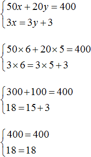
Let's return to the very first system, which described how many cakes and cups of coffee the student bought. The solution of this system was a pair of values (6; 5) .

We multiply both equations included in this system by some numbers. Let's say we multiply the first equation by 2 and the second by 3

The result is a system
The solution to this system is still the pair of values (6; 5)

This means that the equations included in the system can be reduced to a form suitable for applying the addition method.

Back to the system , which we could not solve by the addition method.

Multiply the first equation by 6 and the second by −2

Then we get the following system:

We add the equations included in this system. Addition of components 12 x and -12 x will result in 0, addition 18 y and 4 y will give 22 y, and adding 108 and −20 gives 88. Then you get the equation 22 y= 88 , hence y = 4 .

If at first it’s hard to add equations in your mind, then you can write down how the left side of the first equation is added to the left side of the second equation, and the right side of the first equation to the right side of the second equation:

Knowing that the value of the variable y is 4, you can find the value x. Substitute y into one of the equations, for example into the first equation 2 x+ 3y= 18 . Then we get an equation with one variable 2 x+ 12 = 18 . We transfer 12 to the right side, changing the sign, we get 2 x= 6 , hence x = 3 .

Example 4. Solve the following system of equations using the addition method:

Multiply the second equation by −1. Then the system will take the following form:

Let's add both equations. Addition of components x and −x will result in 0, addition 5 y and 3 y will give 8 y, and adding 7 and 1 gives 8. The result is equation 8 y= 8 , whose root is 1. Knowing that the value y is 1, you can find the value x .

Substitute y into the first equation, we get x+ 5 = 7 , hence x= 2

Example 5. Solve the following system of equations using the addition method:

It is desirable that the terms containing the same variables are located one under the other. Therefore, in the second equation, the terms 5 y and −2 x change places. As a result, the system will take the form:

Multiply the second equation by 3. Then the system will take the form:

Now let's add both equations. As a result of addition, we get equation 8 y= 16 , whose root is 2.

Substitute y into the first equation, we get 6 x− 14 = 40 . We transfer the term −14 to the right side, changing the sign, we get 6 x= 54 . From here x= 9.

Example 6. Solve the following system of equations using the addition method:

Let's get rid of fractions. Multiply the first equation by 36 and the second by 12

In the resulting system the first equation can be multiplied by −5 and the second by 8

Let's add the equations in the resulting system. Then we get the simplest equation −13 y= −156 . From here y= 12 . Substitute y into the first equation and find x

Example 7. Solve the following system of equations using the addition method:

We bring both equations to normal form. Here it is convenient to apply the rule of proportion in both equations. If in the first equation the right side is represented as , and the right side of the second equation as , then the system will take the form:

We have a proportion. We multiply its extreme and middle terms. Then the system will take the form:

We multiply the first equation by −3, and open the brackets in the second:

Now let's add both equations. As a result of adding these equations, we get an equality, in both parts of which there will be zero:

It turns out that the system has an infinite number of solutions.

But we cannot simply take arbitrary values from the sky for x and y. We can specify one of the values, and the other will be determined depending on the value we specify. For example, let x= 2 . Substitute this value into the system:

As a result of solving one of the equations, the value for y, which will satisfy both equations:

The resulting pair of values (2; −2) will satisfy the system:

Let's find another pair of values. Let x= 4. Substitute this value into the system:

It can be determined by eye that y equals zero. Then we get a pair of values (4; 0), which satisfies our system:

Example 8. Solve the following system of equations using the addition method:

Multiply the first equation by 6 and the second by 12

Let's rewrite what's left:

Multiply the first equation by −1. Then the system will take the form:

Now let's add both equations. As a result of addition, equation 6 is formed b= 48 , whose root is 8. Substitute b into the first equation and find a

System of linear equations with three variables

A linear equation with three variables includes three variables with coefficients, as well as an intercept. In canonical form, it can be written as follows:

ax + by + cz = d

This equation has an infinite number of solutions. Giving two variables various meanings, you can find the third value. The solution in this case is the triple of values ( x; y; z) which turns the equation into an identity.

If variables x, y, z are interconnected by three equations, then a system of three linear equations with three variables is formed. To solve such a system, you can apply the same methods that apply to linear equations with two variables: the substitution method and the addition method.

Example 1. Solve the following system of equations using the substitution method:

We express in the third equation x. Then the system will take the form:

Now let's do the substitution. Variable x is equal to the expression 3 − 2y − 2z . Substitute this expression into the first and second equations:

Let's open the brackets in both equations and give like terms:

We have arrived at a system of linear equations with two variables. In this case, it is convenient to apply the addition method. As a result, the variable y will disappear and we can find the value of the variable z

Now let's find the value y. For this, it is convenient to use the equation − y+ z= 4. Substitute the value z

Now let's find the value x. For this, it is convenient to use the equation x= 3 − 2y − 2z . Substitute the values into it y and z

Thus, the triple of values (3; −2; 2) is the solution to our system. By checking, we make sure that these values satisfy the system:

Example 2. Solve the system by addition method

Let's add the first equation with the second multiplied by −2.

If the second equation is multiplied by −2, then it will take the form −6x+ 6y- 4z = −4 . Now add it to the first equation:

We see that as a result of elementary transformations, the value of the variable was determined x. It is equal to one.

Let's go back to the main system. Let's add the second equation with the third multiplied by −1. If the third equation is multiplied by −1, then it will take the form −4x + 5y − 2z = −1 . Now add it to the second equation:

Got the equation x - 2y= −1 . Substitute the value into it x which we found earlier. Then we can determine the value y

We now know the values x and y. This allows you to determine the value z. We use one of the equations included in the system:

Thus, the triple of values (1; 1; 1) is the solution to our system. By checking, we make sure that these values satisfy the system:

Tasks for compiling systems of linear equations

The task of compiling systems of equations is solved by introducing several variables. Next, equations are compiled based on the conditions of the problem. From the compiled equations, they form a system and solve it. Having solved the system, it is necessary to check whether its solution satisfies the conditions of the problem.

Task 1. A Volga car left the city for the collective farm. She returned back along another road, which was 5 km shorter than the first. In total, the car drove 35 km both ways. How many kilometers is each road long?

Solution

Let x- length of the first road, y- the length of the second. If the car drove 35 km both ways, then the first equation can be written as x+ y= 35. This equation describes the sum of the lengths of both roads.

It is said that the car was returning back along the road, which was shorter than the first one by 5 km. Then the second equation can be written as x− y= 5. This equation shows that the difference between the lengths of the roads is 5 km.

Or the second equation can be written as x= y+ 5 . We will use this equation.

Since the variables x and y in both equations denote the same number, then we can form a system from them:

Let's solve this system using one of the previously studied methods. In this case, it is convenient to use the substitution method, since in the second equation the variable x already expressed.

Substitute the second equation into the first and find y

Substitute the found value y into the second equation x= y+ 5 and find x

The length of the first road was denoted by the variable x. Now we have found its meaning. Variable x is 20. So the length of the first road is 20 km.

And the length of the second road was indicated by y. The value of this variable is 15. So the length of the second road is 15 km.

Let's do a check. First, let's make sure that the system is solved correctly:

Now let's check whether the solution (20; 15) satisfies the conditions of the problem.

It was said that in total the car drove 35 km both ways. We add up the lengths of both roads and make sure that the solution (20; 15) satisfies this condition: 20 km + 15 km = 35 km

Next condition: the car returned back along another road, which was 5 km shorter than the first . We see that the solution (20; 15) also satisfies this condition, since 15 km is shorter than 20 km by 5 km: 20 km − 15 km = 5 km

When compiling a system, it is important that the variables denote the same numbers in all equations included in this system.

So our system contains two equations. These equations in turn contain the variables x and y, which denote the same numbers in both equations, namely the lengths of roads equal to 20 km and 15 km.

Task 2. Oak and pine sleepers were loaded onto the platform, a total of 300 sleepers. It is known that all oak sleepers weighed 1 ton less than all pine sleepers. Determine how many oak and pine sleepers there were separately, if each oak sleeper weighed 46 kg, and each pine sleeper 28 kg.

Solution

Let x oak and y pine sleepers were loaded onto the platform. If there were 300 sleepers in total, then the first equation can be written as x+y = 300 .

All oak sleepers weighed 46 x kg, and pine weighed 28 y kg. Since oak sleepers weighed 1 ton less than pine sleepers, the second equation can be written as 28y- 46x= 1000 . This equation shows that the mass difference between oak and pine sleepers is 1000 kg.

Tons have been converted to kilograms because the mass of oak and pine sleepers is measured in kilograms.

As a result, we obtain two equations that form the system

Let's solve this system. Express in the first equation x. Then the system will take the form:

Substitute the first equation into the second and find y

Substitute y into the equation x= 300 − y and find out what x

This means that 100 oak and 200 pine sleepers were loaded onto the platform.

Let's check whether the solution (100; 200) satisfies the conditions of the problem. First, let's make sure that the system is solved correctly:

It was said that there were 300 sleepers in total. We add up the number of oak and pine sleepers and make sure that the solution (100; 200) satisfies this condition: 100 + 200 = 300.

Next condition: all oak sleepers weighed 1 ton less than all pine . We see that the solution (100; 200) also satisfies this condition, since 46 × 100 kg of oak sleepers are lighter than 28 × 200 kg of pine sleepers: 5600 kg − 4600 kg = 1000 kg.

Task 3. We took three pieces of an alloy of copper and nickel in ratios of 2: 1, 3: 1 and 5: 1 by weight. Of these, a piece weighing 12 kg was fused with a ratio of copper and nickel content of 4: 1. Find the mass of each original piece if the mass of the first of them is twice the mass of the second.

where x* - one of the solutions of the inhomogeneous system (2) (for example (4)), (E−A + A) forms the kernel (zero space) of the matrix A.

Let's make a skeletal decomposition of the matrix (E−A + A):

E−A + A=Q S

where Q n×n−r- rank matrix (Q)=n−r, S n−r×n-rank matrix (S)=n−r.

Then (13) can be written in the following form:

x=x*+Qk, ∀ k ∈ R n-r .

where k=Sz.

So, general solution procedure system of linear equations using pseudo inverse matrix can be presented in the following form:

Calculate the pseudoinverse matrix A + .
We calculate a particular solution of the inhomogeneous system of linear equations (2): x*=A + b.
We check the compatibility of the system. For this we calculate AA + b. If a AA + b≠b, then the system is inconsistent. Otherwise, we continue the procedure.
vyssylyaem E−A+A.
Doing a skeletal decomposition E−A + A=Q·S.
Building a Solution

x=x*+Qk, ∀ k ∈ R n-r .

Solving a system of linear equations online

The online calculator allows you to find the general solution of a system of linear equations with detailed explanations.

§one. Systems of linear equations.

view system

called a system m linear equations with n unknown.

Here
- unknown, - coefficients for unknowns,
- free members of the equations.

If all free terms of the equations are equal to zero, the system is called homogeneous.Decision system is called a set of numbers
, when substituting them into the system instead of unknowns, all equations turn into identities. The system is called joint if it has at least one solution. A joint system with a unique solution is called certain. The two systems are called equivalent if the sets of their solutions are the same.

System (1) can be represented in matrix form using the equation

(2)

§2. Compatibility of systems of linear equations.

We call the extended matrix of system (1) the matrix

Kronecker - Capelli theorem. System (1) is consistent if and only if the rank of the system matrix is equal to the rank of the extended matrix:

§3. Systems solutionn linear equations withn unknown.

Consider an inhomogeneous system n linear equations with n unknown:

(3)

Cramer's theorem.If the main determinant of the system (3)
, then the system has a unique solution determined by the formulas:

those.
,

where - the determinant obtained from the determinant replacement th column to the column of free members.

If a
, and at least one of ≠0, then the system has no solutions.

If a
, then the system has infinitely many solutions.

System (3) can be solved using its matrix notation (2). If the rank of the matrix BUT equals n, i.e.
, then the matrix BUT has an inverse
. Multiplying the matrix equation
to matrix
on the left, we get:

The last equality expresses a way to solve systems of linear equations using an inverse matrix.

Example. Solve the system of equations using the inverse matrix.

Solution. Matrix
non-degenerate, because
, so there is an inverse matrix. Let's calculate the inverse matrix:
.

Exercise. Solve the system by Cramer's method.

§four. Solution of arbitrary systems of linear equations.

Let an inhomogeneous system of linear equations of the form (1) be given.

Let us assume that the system is consistent, i.e. the condition of the Kronecker-Capelli theorem is fulfilled:
. If the rank of the matrix
(to the number of unknowns), then the system has a unique solution. If a
, then the system has infinitely many solutions. Let's explain.

Let the rank of the matrix r(A)= r< n. Because the
, then there exists some nonzero minor of order r. Let's call it the basic minor. Unknowns whose coefficients form basic minor, we will call the basic variables. The remaining unknowns are called free variables. We rearrange the equations and renumber the variables so that this minor is located in the upper left corner of the system matrix:

First r rows are linearly independent, the rest are expressed through them. Therefore, these lines (equations) can be discarded. We get:

We give free variables arbitrary numerical values: . We leave only the basic variables on the left side, and move the free variables to the right side.

Got a system r linear equations with r unknown, whose determinant is different from 0. It has a unique solution.

This system is called the general solution of the system of linear equations (1). Otherwise: the expression of basic variables in terms of free ones is called common solution systems. From it you can get an infinite number private decisions, giving free variables arbitrary values. A particular solution obtained from a general one at zero values of the free variables is called basic solution. The number of different basic solutions does not exceed
. A basic solution with non-negative components is called pivotal system solution.

Example.

,r=2.

Variables
- basic,
- free.

Let's add the equations; express
through
:

- common decision.

- private solution
.

- basic solution, basic.

§5. Gauss method.

The Gauss method is a universal method for studying and solving arbitrary systems of linear equations. It consists in bringing the system to a diagonal (or triangular) form by sequential elimination of unknowns using elementary transformations that do not violate the equivalence of systems. A variable is considered excluded if it is contained in only one equation of the system with a coefficient of 1.

Elementary transformations systems are:

Multiplying an equation by a non-zero number;

Adding an equation multiplied by any number with another equation;

Rearrangement of equations;

Dropping the equation 0 = 0.

Elementary transformations can be performed not on equations, but on extended matrices of the resulting equivalent systems.

Example.

Solution. We write the extended matrix of the system:

Performing elementary transformations, we bring the left side of the matrix to the unit form: we will create units on the main diagonal, and zeros outside it.

Comment. If, when performing elementary transformations, an equation of the form 0 = to(where to0), then the system is inconsistent.

The solution of systems of linear equations by the method of successive elimination of unknowns can be formalized in the form tables.

The left column of the table contains information about the excluded (basic) variables. The remaining columns contain the coefficients of the unknowns and the free terms of the equations.

The expanded matrix of the system is written into the source table. Next, proceed to the implementation of the Jordan transformations:

1. Choose a variable , which will become the basis. The corresponding column is called the key column. Choose an equation in which this variable will remain, being excluded from other equations. The corresponding table row is called the key row. Coefficient The , standing at the intersection of the key row and the key column, is called the key.

2. Elements of the key string are divided by the key element.

3. The key column is filled with zeros.

4. The remaining elements are calculated according to the rectangle rule. They make up a rectangle, at opposite vertices of which there are a key element and a recalculated element; from the product of the elements on the diagonal of the rectangle with the key element, the product of the elements of another diagonal is subtracted, the resulting difference is divided by the key element.

Example. Find the general solution and the basic solution of the system of equations:

Solution.

General solution of the system:

Basic solution:
.

A one-time substitution transformation allows one to go from one basis of the system to another: instead of one of the main variables, one of the free variables is introduced into the basis. To do this, a key element is selected in the free variable column and transformations are performed according to the above algorithm.

§6. Finding support solutions

The reference solution of a system of linear equations is a basic solution that does not contain negative components.

The support solutions of the system are found by the Gauss method under the following conditions.

1. In the original system, all free terms must be non-negative:
.

2. The key element is chosen among positive coefficients.

3. If the variable introduced into the basis has several positive coefficients, then the key string is the one in which the ratio of the free term to the positive coefficient is the smallest.

Remark 1. If, in the process of eliminating the unknowns, an equation appears in which all coefficients are nonpositive, and the free term
, then the system has no non-negative solutions.

Remark 2. If there is not a single positive element in the columns of coefficients for free variables, then the transition to another reference solution is impossible.

Example.

Solution. A= . Find r(A). Because matrix A has order 3x4, then highest order minors is 3. In this case, all third-order minors are equal to zero (check it yourself). Means, r(А)< 3. Возьмем главный basic minor = -5-4 = -9 ≠ 0. Hence r(A) =2.

Consider matrix FROM = .

Minor third order ≠ 0. Hence, r(C) = 3.

Since r(A) ≠ r(C) , then the system is inconsistent.

Example 2 Determine the compatibility of the system of equations

Solve this system if it is consistent.

Solution.

A = , C = . Obviously, r(А) ≤ 3, r(C) ≤ 4. Since detC = 0, then r(C)< 4. Consider minor third order, located in the upper left corner of the matrix A and C: = -23 ≠ 0. Hence, r(A) = r(C) = 3.

Number unknown in the system n=3. So the system has a unique solution. In this case, the fourth equation is the sum of the first three and can be ignored.

According to Cramer's formulas we get x 1 = -98/23, x 2 = -47/23, x 3 = -123/23.

2.4. Matrix method. Gauss method

system n linear equations With n unknowns can be solved matrix method according to the formula X \u003d A -1 B (for Δ ≠ 0), which is obtained from (2) by multiplying both parts by A -1 .

Example 1. Solve a system of equations

by the matrix method (in Section 2.2 this system was solved using the Cramer formulas)

Solution. Δ=10 ≠ 0 A = - nonsingular matrix.

= (verify this for yourself by doing the necessary calculations).

A -1 \u003d (1 / Δ) x \u003d .

X \u003d A -1 B \u003d x= .

Answer: .

From a practical point of view matrix method and formulas Kramer are associated with a large amount of computation, so preference is given to Gauss method, which consists in sequential exclusion unknown. To do this, the system of equations is reduced to an equivalent system with a triangular augmented matrix (all elements below the main diagonal are equal to zero). These actions are called direct move. From the resulting triangular system, the variables are found using successive substitutions (backward).

Example 2. Solve the system using the Gauss method

(This system was solved above using the Cramer formula and the matrix method).

Solution.

Direct move. We write the augmented matrix and, using elementary transformations, bring it to a triangular form:

~ ~ ~ ~ .

Get system

Reverse move. From the last equation we find X 3 = -6 and substitute this value into the second equation:

X 2 = - 11/2 - 1/4X 3 = - 11/2 - 1/4(-6) = - 11/2 + 3/2 = -8/2 = -4.

X 1 = 2 -X 2 + X 3 = 2+4-6 = 0.

Answer: .

2.5. General solution of a system of linear equations

Let a system of linear equations be given = b i(i=). Let r(A) = r(C) = r, i.e. the system is collaborative. Any non-zero minor of order r is basic minor. Without loss of generality, we assume that the basis minor is located in the first r (1 ≤ r ≤ min(m,n)) rows and columns of the matrix A. Discarding the last m-r equations system, we write a shortened system:

which is equivalent to the original. Let's name the unknowns x 1 ,….x r basic , and x r +1 ,…, x r free and move the terms containing the free unknowns to the right side of the equations of the truncated system. We get the system with respect to the basic unknowns:

which for each set of values of free unknowns x r +1 \u003d C 1, ..., x n \u003d C n-r has the only solution x 1 (C 1, ..., C n-r), ..., x r (C 1, ..., C n-r), found by Cramer's rule.

Appropriate decision shortened, and hence the original system has the form:

Х(С 1 ,…, С n-r) = - general solution of the system.

If we give some numerical values to the free unknowns in the general solution, then we get the solution linear system, called private .

Example. Establish compatibility and find the overall solution of the system

Solution. A = , С = .

So how r(A)= r(C) = 2 (see for yourself), then the original system is compatible and has an infinite number of solutions (since r< 4).

To investigate a system of linear agebraic equations (SLAE) for compatibility means to find out whether this system has solutions or not. Well, if there are solutions, then indicate how many of them.

We will need information from the topic "System of linear algebraic equations. Basic terms. Matrix notation". In particular, such concepts as the matrix of the system and the extended matrix of the system are needed, since the formulation of the Kronecker-Capelli theorem is based on them. As usual, the matrix of the system will be denoted by the letter $A$, and the extended matrix of the system by the letter $\widetilde(A)$.

Kronecker-Capelli theorem

Linear system algebraic equations is consistent if and only if the rank of the system matrix is equal to the rank of the extended matrix of the system, i.e. $\rank A=\rang\widetilde(A)$.

Let me remind you that a system is called joint if it has at least one solution. The Kronecker-Capelli theorem says this: if $\rang A=\rang\widetilde(A)$, then there is a solution; if $\rang A\neq\rang\widetilde(A)$, then this SLAE has no solutions (is inconsistent). The answer to the question about the number of these solutions is given by a corollary of the Kronecker-Capelli theorem. The statement of the corollary uses the letter $n$, which is equal to the number of variables in the given SLAE.

Corollary from the Kronecker-Capelli theorem

If $\rang A\neq\rang\widetilde(A)$, then the SLAE is inconsistent (has no solutions).
If $\rang A=\rang\widetilde(A)< n$, то СЛАУ является неопределённой (имеет бесконечное количество решений).
If $\rang A=\rang\widetilde(A) = n$, then the SLAE is definite (it has exactly one solution).

Note that the formulated theorem and its corollary do not indicate how to find the solution to the SLAE. With their help, you can only find out whether these solutions exist or not, and if they exist, then how many.

Example #1

Explore SLAE $ \left \(\begin(aligned) & -3x_1+9x_2-7x_3=17;\\ & -x_1+2x_2-4x_3=9;\\ & 4x_1-2x_2+19x_3=-42. \end(aligned )\right.$ for consistency If the SLAE is consistent, indicate the number of solutions.

To find out the existence of solutions to a given SLAE, we use the Kronecker-Capelli theorem. We need the matrix of the system $A$ and the extended matrix of the system $\widetilde(A)$, we write them down:

$$ A=\left(\begin(array) (ccc) -3 & 9 & -7 \\ -1 & 2 & -4 \\ 4 & -2 & 19 \end(array) \right);\; \widetilde(A)=\left(\begin(array) (ccc|c) -3 & 9 &-7 & 17 \\ -1 & 2 & -4 & 9\\ 4 & -2 & 19 & -42 \end(array)\right). $$

We need to find $\rang A$ and $\rang\widetilde(A)$. There are many ways to do this, some of which are listed in the Matrix Rank section. Usually, two methods are used to study such systems: "Calculation of the rank of a matrix by definition" or "Calculation of the rank of a matrix by the method of elementary transformations".

Method number 1. Calculation of ranks by definition.

According to the definition, the rank is the highest order of the minors of the matrix , among which there is at least one other than zero. Usually, the study begins with the first-order minors, but here it is more convenient to proceed immediately to the calculation of the third-order minor of the matrix $A$. The elements of the third-order minor are at the intersection of three rows and three columns of the matrix under consideration. Since the matrix $A$ contains only 3 rows and 3 columns, the third order minor of the matrix $A$ is the determinant of the matrix $A$, i.e. $\DeltaA$. To calculate the determinant, we apply formula No. 2 from the topic "Formulas for calculating second and third order determinants":

$$ \Delta A=\left| \begin(array) (ccc) -3 & 9 & -7 \\ -1 & 2 & -4 \\ 4 & -2 & 19 \end(array) \right|=-21. $$

So, there is a third-order minor of the matrix $A$, which is not equal to zero. A 4th-order minor cannot be composed, since it requires 4 rows and 4 columns, and the matrix $A$ has only 3 rows and 3 columns. So, the highest order of minors of the matrix $A$, among which there is at least one non-zero one, is equal to 3. Therefore, $\rang A=3$.

We also need to find $\rang\widetilde(A)$. Let's look at the structure of the $\widetilde(A)$ matrix. Up to the line in the matrix $\widetilde(A)$ there are elements of the matrix $A$, and we found out that $\Delta A\neq 0$. Therefore, the matrix $\widetilde(A)$ has a third-order minor that is not equal to zero. We cannot compose fourth-order minors of the matrix $\widetilde(A)$, so we conclude: $\rang\widetilde(A)=3$.

Since $\rang A=\rang\widetilde(A)$, according to the Kronecker-Capelli theorem, the system is consistent, i.e. has a solution (at least one). To indicate the number of solutions, we take into account that our SLAE contains 3 unknowns: $x_1$, $x_2$ and $x_3$. Since the number of unknowns is $n=3$, we conclude: $\rang A=\rang\widetilde(A)=n$, therefore, according to the corollary of the Kronecker-Capelli theorem, the system is definite, i.e. has a unique solution.

Problem solved. What are the disadvantages and advantages of this method? First, let's talk about the pros. First, we needed to find only one determinant. After that, we immediately made a conclusion about the number of solutions. Usually, in standard typical calculations, systems of equations are given that contain three unknowns and have a single solution. For such systems this method very convenient, because we know in advance that there is a solution (otherwise there would be no example in a typical calculation). Those. it only remains for us to show that there is a solution to the most fast way. Secondly, the calculated value of the system matrix determinant (i.e. $\Delta A$) will come in handy later: when we start solving the given system using the Cramer method or using the inverse matrix .

However, by definition, the method of calculating the rank is undesirable if the system matrix $A$ is rectangular. In this case, it is better to apply the second method, which will be discussed below. Besides, if $\Delta A=0$, then we will not be able to say anything about the number of solutions for a given inhomogeneous SLAE. Maybe SLAE has an infinite number of solutions, or maybe none. If $\Delta A=0$, then additional research is required, which is often cumbersome.

Summarizing what has been said, I note that the first method is good for those SLAEs whose system matrix is square. At the same time, the SLAE itself contains three or four unknowns and is taken from standard standard calculations or control works.

Method number 2. Calculation of the rank by the method of elementary transformations.

This method is described in detail in the corresponding topic. We will calculate the rank of the matrix $\widetilde(A)$. Why matrices $\widetilde(A)$ and not $A$? The point is that the matrix $A$ is a part of the matrix $\widetilde(A)$, so by calculating the rank of the matrix $\widetilde(A)$ we will simultaneously find the rank of the matrix $A$.

\begin(aligned) &\widetilde(A) =\left(\begin(array) (ccc|c) -3 & 9 &-7 & 17 \\ -1 & 2 & -4 & 9\\ 4 & - 2 & 19 & -42 \end(array) \right) \rightarrow \left|\text(swap first and second lines)\right| \rightarrow \\ &\rightarrow \left(\begin(array) (ccc|c) -1 & 2 & -4 & 9 \\ -3 & 9 &-7 & 17\\ 4 & -2 & 19 & - 42 \end(array) \right) \begin(array) (l) \phantom(0) \\ II-3\cdot I\\ III+4\cdot I \end(array) \rightarrow \left(\begin (array) (ccc|c) -1 & 2 & -4 & 9 \\ 0 & 3 &5 & -10\\ 0 & 6 & 3 & -6 \end(array) \right) \begin(array) ( l) \phantom(0) \\ \phantom(0)\\ III-2\cdot II \end(array)\rightarrow\\ &\rightarrow \left(\begin(array) (ccc|c) -1 & 2 & -4 & 9 \\ 0 & 3 &5 & -10\\ 0 & 0 & -7 & 14 \end(array) \right) \end(aligned)

We have reduced the matrix $\widetilde(A)$ to a trapezoidal form . On the main diagonal of the resulting matrix $\left(\begin(array) (ccc|c) -1 & 2 & -4 & 9 \\ 0 & 3 &5 & -10\\ 0 & 0 & -7 & 14 \end( array) \right)$ contains three non-zero elements: -1, 3 and -7. Conclusion: the rank of the matrix $\widetilde(A)$ is 3, i.e. $\rank\widetilde(A)=3$. Making transformations with the elements of the matrix $\widetilde(A)$, we simultaneously transformed the elements of the matrix $A$ located before the line. The matrix $A$ is also trapezoidal: $\left(\begin(array) (ccc) -1 & 2 & -4 \\ 0 & 3 &5 \\ 0 & 0 & -7 \end(array) \right )$. Conclusion: the rank of the matrix $A$ is also equal to 3, i.e. $\rank A=3$.

Since $\rang A=\rang\widetilde(A)$, according to the Kronecker-Capelli theorem, the system is consistent, i.e. has a solution. To indicate the number of solutions, we take into account that our SLAE contains 3 unknowns: $x_1$, $x_2$ and $x_3$. Since the number of unknowns is $n=3$, we conclude: $\rang A=\rang\widetilde(A)=n$, therefore, according to the corollary of the Kronecker-Capelli theorem, the system is defined, i.e. has a unique solution.

What are the advantages of the second method? The main advantage is its versatility. It doesn't matter to us whether the matrix of the system is square or not. In addition, we have actually carried out transformations of the Gauss method forward. There are only a couple of steps left, and we could get the solution of this SLAE. To be honest, I like the second way more than the first, but the choice is a matter of taste.

Answer: The given SLAE is consistent and defined.

Example #2

Explore SLAE $ \left\( \begin(aligned) & x_1-x_2+2x_3=-1;\\ & -x_1+2x_2-3x_3=3;\\ & 2x_1-x_2+3x_3=2;\\ & 3x_1- 2x_2+5x_3=1;\\ & 2x_1-3x_2+5x_3=-4.\end(aligned) \right.$ for consistency.

We will find the ranks of the system matrix and the extended matrix of the system by the method of elementary transformations. Extended system matrix: $\widetilde(A)=\left(\begin(array) (ccc|c) 1 & -1 & 2 & -1\\ -1 & 2 & -3 & 3 \\ 2 & -1 & 3 & 2 \\ 3 & -2 & 5 & 1 \\ 2 & -3 & 5 & -4 \end(array) \right)$. Let's find the required ranks by transforming the augmented matrix of the system:

The extended matrix of the system is reduced to a stepped form. If the matrix is reduced to a stepped form, then its rank is equal to the number of non-zero rows. Therefore, $\rank A=3$. The matrix $A$ (up to the line) is reduced to a trapezoidal form and its rank is equal to 2, $\rang A=2$.

Since $\rang A\neq\rang\widetilde(A)$, then, according to the Kronecker-Capelli theorem, the system is inconsistent (ie, has no solutions).

Answer: The system is inconsistent.

Example #3

Explore SLAE $ \left\( \begin(aligned) & 2x_1+7x_3-5x_4+11x_5=42;\\ & x_1-2x_2+3x_3+2x_5=17;\\ & -3x_1+9x_2-11x_3-7x_5=-64 ;\\ & -5x_1+17x_2-16x_3-5x_4-4x_5=-90;\\ & 7x_1-17x_2+23x_3+15x_5=132. \end(aligned) \right.$ for compatibility.

The extended system matrix is: $\widetilde(A)=\left(\begin(array) (ccccc|c) 2 & 0 & 7 & -5 & 11 & 42\\ 1 & -2 & 3 & 0 & 2 & 17 \\ -3 & 9 & -11 & 0 & -7 & -64 \\ -5 & 17 & -16 & -5 & -4 & -90 \\ 7 & -17 & 23 & 0 & 15 & 132 \end(array)\right)$. Swap the first and second rows of this matrix so that the first element of the first row is one: $\left(\begin(array) (ccccc|c) 1 & -2 & 3 & 0 & 2 & 17\\ 2 & 0 & 7 & -5 & 11 & 42 \\ -3 & 9 & -11 & 0 & -7 & -64 \\ -5 & 17 & -16 & -5 & -4 & -90 \\ 7 & -17 & 23 & 0 & 15 & 132 \end(array) \right)$.

We have reduced the extended matrix of the system and the matrix of the system itself to a trapezoidal form. The rank of the extended matrix of the system is equal to three, the rank of the matrix of the system is also equal to three. Since the system contains $n=5$ unknowns, i.e. $\rang\widetilde(A)=\rank A< n$, то согласно следствия из теоремы Кронекера-Капелли this system is indefinite, i.e. has an infinite number of solutions.

Answer: the system is indeterminate.

In the second part, we will analyze examples that are often included in typical calculations or test papers in higher mathematics: a study on the compatibility and solution of SLAE depending on the values of the parameters included in it.