Test: Chi-square distribution and its application. Pearson's goodness-of-fit test χ2 (Chi-square)
Pearson's chi-square test is a non-parametric method that allows you to assess the significance of differences between the actual (revealed as a result of the study) number of outcomes or qualitative characteristics of the sample that fall into each category and the theoretical number that can be expected in the studied groups if the null hypothesis is true. In simpler terms, the method allows you to evaluate the statistical significance of differences between two or more relative indicators (frequencies, shares).
1. History of the development of the χ 2 criterion
The chi-square test for the analysis of contingency tables was developed and proposed in 1900 by an English mathematician, statistician, biologist and philosopher, the founder of mathematical statistics and one of the founders of biometrics Karl Pearson(1857-1936).
2. What is Pearson's χ 2 criterion used for?
The chi-square test can be applied in the analysis contingency tables containing information about the frequency of outcomes depending on the presence of a risk factor. For example, four-field contingency table as follows:
| Exodus is (1) | No exit (0) | Total | |
| There is a risk factor (1) | A | B | A+B |
| No risk factor (0) | C | D | C+D |
| Total | A+C | B+D | A+B+C+D |
How to fill in such a contingency table? Let's consider a small example.
A study is underway on the effect of smoking on the risk of developing arterial hypertension. For this, two groups of subjects were selected - the first included 70 people who smoke at least 1 pack of cigarettes daily, the second - 80 non-smokers of the same age. In the first group, 40 people had high blood pressure. In the second - arterial hypertension was observed in 32 people. Accordingly, normal blood pressure in the group of smokers was in 30 people (70 - 40 = 30) and in the group of non-smokers - in 48 (80 - 32 = 48).
We fill in the four-field contingency table with the initial data:
In the resulting contingency table, each line corresponds to a specific group of subjects. Columns - show the number of persons with arterial hypertension or with normal blood pressure.
The challenge for the researcher is: are there statistically significant differences between the frequency of people with blood pressure among smokers and non-smokers? You can answer this question by calculating Pearson's chi-square test and comparing the resulting value with the critical one.
3. Conditions and restrictions on the use of Pearson's chi-square test
- Comparable indicators should be measured in nominal scale(for example, the patient's gender - male or female) or in ordinal(for example, the degree of arterial hypertension, taking values from 0 to 3).
- This method allows analysis not only of four-field tables, when both the factor and the outcome are binary variables, that is, they have only two possible values (for example, male or female, the presence or absence of a certain disease in history ...). Pearson's chi-square test can also be used in the case of the analysis of multi-field tables, when the factor and (or) outcome take three or more values.
- The matched groups should be independent, i.e. the chi-square test should not be used when comparing before-after observations. McNemar test(when comparing two related populations) or calculated Q-test Cochran(in case of comparing three or more groups).
- When analyzing four-field tables expected values in each of the cells must be at least 10. In the event that in at least one cell the expected phenomenon takes a value from 5 to 9, the chi-square test must be calculated with Yates correction. If in at least one cell the expected phenomenon is less than 5, then the analysis should use Fisher's exact test.
- In the case of analysis of multi-field tables, the expected number of observations should not take values less than 5 in more than 20% of the cells.
4. How to calculate Pearson's chi-square test?
To calculate the chi-square test, you must:

This algorithm is applicable for both four-field and multi-field tables.
5. How to interpret the value of Pearson's chi-square test?
In the event that the obtained value of the criterion χ 2 is greater than the critical one, we conclude that there is a statistical relationship between the studied risk factor and the outcome at the appropriate level of significance.
6. An example of calculating the Pearson chi-square test
Let us determine the statistical significance of the influence of the smoking factor on the incidence of arterial hypertension according to the table above:
- We calculate the expected values for each cell:
- Find the value of Pearson's chi-square test:
χ 2 \u003d (40-33.6) 2 / 33.6 + (30-36.4) 2 / 36.4 + (32-38.4) 2 / 38.4 + (48-41.6) 2 / 41.6 \u003d 4.396.
- The number of degrees of freedom f = (2-1)*(2-1) = 1. We find the critical value of the Pearson chi-square test from the table, which, at a significance level of p=0.05 and the number of degrees of freedom 1, is 3.841.
- We compare the obtained value of the chi-square test with the critical one: 4.396 > 3.841, therefore, the dependence of the incidence of arterial hypertension on the presence of smoking is statistically significant. The significance level of this relationship corresponds to p<0.05.
This post does not answer how to calculate the Chi squared criterion in principle, its purpose is to show how you can automate chi square calculation in excel, what functions for calculating the Chi square criterion are there. For SPSS or the R program is not always at hand.
In a sense, this is a reminder and hint to the participants of the Analytics for HR seminar, I hope you use these methods in your work, this post will be another hint.
I do not give the file a download link, but you can just copy the example tables I have provided and run through the data and formulas I have provided
introductory
For example, we want to check the independence (randomness / non-randomness) of the distribution of the results of a corporate survey, where in the rows are the answers to any question of the questionnaire, and in the columns - the distribution by length of service.You enter the Chi squared calculation through the pivot table when your data is summarized in a conjugation table, for example, in this form
Table #1
less than 1 year |
Sum by lines |
|||||
Sum across columns |
HI2.TEST
The CHI2.TEST formula calculates the probability of independence (randomness / non-randomness) of the distribution
The syntax is
CHI2.TEST(actual_interval, expected_interval)
In our case, the actual interval is the contents of the table, i.e.
In our case, CH2.DIST.RT = 0.000466219908895455, as in the CH2.TEST example
Note
This formula for calculating Chi-square in excel is suitable for calculating 2X2 tables, since you yourself consider Chi-square empirical and can enter a correction for continuity into the calculations
Note 2
There is also the HI2.DIS formula (you will inevitably see it in excel) - it calculates the left-handed probability (if it’s simple, then the left-handed one is considered as 1 - right-handed, i.e. we just flip the formula, that’s why I don’t give it in the calculations Chi squared, in our example CHI2.DIST = 0.999533780091105.Total CH2.DIST + CH2.DIST.RT = 1.
chi2.ex.ph
Returns the reciprocal of the right-hand probability of the chi-squared distribution (or just the chi-squared value for a given probability level and number of degrees of freedom)
Synaxis
XI2.INV.RT(probability, degrees_of_freedom)
Conclusion
To be honest, I don't know exactly how the results obtained chi square calculations in excel differ from the results of calculating Chi-square in SPSS. I understand exactly. which are different, if only because when Chi is independently calculated, the squared values are rounded off and a certain number of decimal places are lost. But I don't think it's critical. I recommend only to be insured in the case when the probability of the Chi-squared distribution is close to the threshold (p-value) of 0.05.
It's not great that the correction for continuity is not taken into account - we calculate a lot in 2X2 tables. Therefore, we almost do not achieve optimization in the case of calculating 2X2 tables
Well, nevertheless, I think that the above knowledge is enough to make the calculation of Chi square in excel a little faster to save time on more important things.
). The specific formulation of the hypothesis being tested will vary from case to case.
In this post, I will describe how the \(\chi^2\) test works using a (hypothetical) example from immunology. Imagine that we have performed an experiment to determine the effectiveness of suppressing the development of a microbial disease when the appropriate antibodies are introduced into the body. In total, 111 mice were involved in the experiment, which we divided into two groups, including 57 and 54 animals, respectively. The first group of mice was injected with pathogenic bacteria, followed by the introduction of blood serum containing antibodies against these bacteria. Animals from the second group served as controls - they received only bacterial injections. After some time of incubation, it turned out that 38 mice died, and 73 survived. Of the dead, 13 belonged to the first group, and 25 belonged to the second (control). The null hypothesis tested in this experiment can be formulated as follows: the administration of serum with antibodies has no effect on the survival of mice. In other words, we argue that the observed differences in the survival of mice (77.2% in the first group versus 53.7% in the second group) are completely random and are not associated with the action of antibodies.
The data obtained in the experiment can be presented in the form of a table:
Total |
|||
Bacteria + serum |
|||
Only bacteria |
|||
Total |
Tables like this one are called contingency tables. In this example, the table has a dimension of 2x2: there are two classes of objects ("Bacteria + serum" and "Bacteria only"), which are examined according to two criteria ("Dead" and "Survived"). This is the simplest case of a contingency table: of course, both the number of classes under study and the number of features can be larger.
To test the null hypothesis formulated above, we need to know what the situation would be if the antibodies did not really have any effect on the survival of mice. In other words, you need to calculate expected frequencies for the corresponding cells of the contingency table. How to do it? A total of 38 mice died in the experiment, which is 34.2% of the total number of animals involved. If the introduction of antibodies does not affect the survival of mice, the same percentage of mortality should be observed in both experimental groups, namely 34.2%. Calculating how much is 34.2% of 57 and 54, we get 19.5 and 18.5. These are the expected mortality rates in our experimental groups. The expected survival rates are calculated in a similar way: since 73 mice survived in total, or 65.8% of their total number, the expected survival rates are 37.5 and 35.5. Let's make a new contingency table, now with the expected frequencies:
dead |
Survivors |
Total |
|
Bacteria + serum |
|||
Only bacteria |
|||
Total |
As you can see, the expected frequencies are quite different from the observed ones, i.e. administration of antibodies does seem to have an effect on the survival of mice infected with the pathogen. We can quantify this impression using Pearson's goodness-of-fit test \(\chi^2\):
\[\chi^2 = \sum_()\frac((f_o - f_e)^2)(f_e),\]
where \(f_o\) and \(f_e\) are the observed and expected frequencies, respectively. The summation is performed over all cells of the table. So, for the example under consideration, we have
\[\chi^2 = (13 – 19.5)^2/19.5 + (44 – 37.5)^2/37.5 + (25 – 18.5)^2/18.5 + (29 – 35.5)^2/35.5 = \]
Is \(\chi^2\) large enough to reject the null hypothesis? To answer this question, it is necessary to find the corresponding critical value of the criterion. The number of degrees of freedom for \(\chi^2\) is calculated as \(df = (R - 1)(C - 1)\), where \(R\) and \(C\) are the number of rows and columns in the table conjugacy. In our case \(df = (2 -1)(2 - 1) = 1\). Knowing the number of degrees of freedom, we can now easily find out the critical value \(\chi^2\) using the standard R-function qchisq() :
Thus, for one degree of freedom, the value of the criterion \(\chi^2\) exceeds 3.841 only in 5% of cases. The value we obtained, 6.79, significantly exceeds this critical value, which gives us the right to reject the null hypothesis that there is no relationship between the administration of antibodies and the survival of infected mice. Rejecting this hypothesis, we risk being wrong with a probability of less than 5%.
It should be noted that the above formula for the criterion \(\chi^2\) gives somewhat overestimated values when working with contingency tables of size 2x2. The reason is that the distribution of the \(\chi^2\) criterion itself is continuous, while the frequencies of binary features ("died" / "survived") are discrete by definition. In this regard, when calculating the criterion, it is customary to introduce the so-called. continuity correction, or Yates amendment :
\[\chi^2_Y = \sum_()\frac((|f_o - f_e| - 0.5)^2)(f_e).\]
"s Chi-squared test with Yates" continuity correction data : mice X-squared = 5.7923 , df = 1 , p-value = 0.0161
As you can see, R automatically applies the Yates correction for continuity ( Pearson's Chi-squared test with Yates' continuity correction). The value \(\chi^2\) calculated by the program was 5.79213. We can reject the null hypothesis of no antibody effect at the risk of being wrong with a probability of just over 1% (p-value = 0.0161 ).
The chi-square test of independence is used to determine the relationship between two categorical variables. Examples of pairs of categorical variables are: Marital status vs. The level of employment of the respondent; Dog breed vs. Host Profession, Salary Level vs. Specialization of an engineer, etc. When calculating the criterion of independence, the hypothesis is checked that there is no connection between the variables. We will perform calculations using the MS EXCEL 2010 XI2.TEST () function and the usual formulas.
Suppose we have sample data representing the result of a survey of 500 people. People were asked 2 questions: about their marital status (married, civil marriage, not in a relationship) and their level of employment (full-time, part-time, temporarily unemployed, at home, retired, studying). All answers were placed in the table:
This table is called contingency table of signs(or factorial table, English Contingency table). Elements at the intersection of the rows and columns of the table usually denote O ij (from the English. Observed, i.e. observed, actual frequencies).
We are interested in the question “Does Marital Status Affect Employment?”, i.e. is there a relationship between the two classification methods samples?
At hypothesis testing of this kind, it is usually assumed that null hypothesis states that there is no dependence of methods of classification.
Let's consider the limit cases. An example of a complete dependence of two categorical variables is the following survey result:

In this case, marital status unambiguously determines employment (cf. example file sheet Explanation). Conversely, another survey result is an example of complete independence:

Please note that the percentage of employment in this case does not depend on marital status (the same for married and unmarried). This is exactly the same as the wording null hypothesis. If a null hypothesis is true, then the results of the survey should have been distributed in the table in such a way that the percentage of employees would be the same regardless of marital status. Using this, we compute poll results that match null hypothesis(cm. example file sheet Example).
First, we calculate the probability estimate that the element samples will have a certain employment (see column u i):

where With- the number of columns (columns), equal to the number of levels of the variable "Marital status".
Then we calculate the probability estimate that the element samples will have a certain marital status (see line v j).

where r– the number of rows (rows), equal to the number of levels of the variable "Employment".
The theoretical frequency for each cell E ij (from the English Expected, i.e. the expected frequency) in the case of independent variables is calculated by the formula:
E ij =n* u i * v j

It is known that the statistics X 2 0 for large n has approximately (r-1) (c-1) degrees of freedom (df - degrees of freedom):

If calculated based on samples the value of this statistic is “too large” (greater than the threshold), then null hypothesis rejected. The threshold value is calculated based on , for example, using the formula =XI2.INV.RT(0.05; df) .
Note: Significance level usually taken equal to 0.1; 0.05; 0.01.
At hypothesis testing it is also convenient to calculate , which we compare with significance level. p-meaning calculated using c (r-1)*(c-1)=df degrees of freedom.
If the probability that random value having with (r-1)(c-1) degrees of freedom takes on a value greater than the computed statistic X 2 0 , i.e. P(X 2 (r-1)*(c-1) >X 2 0 ), less significance level, then null hypothesis is rejected.
in MS EXCEL p-value can be calculated using the formula =XI2.DIST.PX(X 2 0 ;df), of course, having computed the value of the X 2 0 statistic immediately before (this is done in the example file). However, it is most convenient to use the XI2.TEST() function. As arguments to this function, references to ranges containing actual (Observed) and calculated theoretical frequencies (Expected) are specified.
If a significance level > p-values, then this is the actual and theoretical frequencies calculated from the assumption of fairness null hypothesis, are seriously different. That's why, null hypothesis must be rejected.
Using the CH2.TEST() function allows you to speed up the procedure hypothesis testing, because no need to calculate value statistics. Now it is enough to compare the result of the function XI2.TEST () with the given significance level.
Note: Function CH2.TEST() , English name CHISQ.TEST appeared in MS EXCEL 2010. Its earlier version CHISQ.TEST() , available in MS EXCEL 2007, has the same functionality. But, as for CHI2.TEST() , the theoretical frequencies must be calculated independently.
Consider the chi-squared distribution. Using the MS EXCEL functionCHI2.DIST() we will construct graphs of the distribution function and probability density, we will explain the application of this distribution for the purposes of mathematical statistics.
Chi-squared distribution (X 2, XI2, EnglishChi- squareddistribution) applied in various methods mathematical statistics:
- when building;
- at ;
- at (whether the empirical data is consistent with our assumption about the theoretical distribution function or not, eng. Goodness-of-fit)
- at (used to determine the relationship between two categorical variables, eng. Chi-square test of association).
Definition: If x 1 , x 2 , …, x n are independent random variables distributed over N(0;1), then the distribution of the random variable Y=x 1 2 + x 2 2 +…+ x n 2 has distribution X 2 with n degrees of freedom.
Distribution X 2 depends on a single parameter called degree of freedom (df, degreesoffreedom). For example, when building number of degrees of freedom is equal to df=n-1, where n is the size samples.
Distribution density X 2
expressed by the formula:
Function Graphs
Distribution X 2 has an asymmetric shape, equal to n, equal to 2n.
AT example file on sheet Graph given distribution density plots probabilities and integral distribution function.

Useful property chi2 distributions
Let x 1 , x 2 , …, x n be independent random variables distributed over normal law with the same parameters μ and σ, and X cf is arithmetic mean these values x.
Then the random variable y equal

It has X 2 -distribution with n-1 degrees of freedom. Using the definition, the above expression can be rewritten as follows:

Consequently, sampling distribution statistics y, with sampling from normal distribution, It has X 2 -distribution with n-1 degrees of freedom.
We will need this property for . Because dispersion can only be a positive number, and X 2 -distribution used to evaluate it y d.b. >0, as stated in the definition.
HI2 distribution in MS EXCEL
In MS EXCEL, starting from version 2010, for X 2 -distributions there is a special function CHISQ.DIST() , the English name is CHISQ.DIST(), which allows you to calculate probability density(see formula above) and (probability that a random variable X having XI2-distribution, takes a value less than or equal to x, P(X<= x}).
Note: Because chi2 distribution is a special case, then the formula =GAMMA.DIST(x,n/2,2,TRUE) for a positive integer n returns the same result as the formula =XI2.DIST(x, n, TRUE) or =1-XI2.DIST.X(x;n) . And the formula =GAMMA.DIST(x,n/2,2,FALSE) returns the same result as the formula =XI2.DIST(x, n, FALSE), i.e. probability density XI2 distributions.
The CH2.DIST.RT() function returns distribution function, more precisely, the right-handed probability, i.e. P(X > x). It is obvious that the equality
=CHI2.DIST.X(x;n)+ CHI2.DIST(x;n;TRUE)=1
because the first term calculates the probability P(X > x), and the second P(X<= x}.
Prior to MS EXCEL 2010, EXCEL had only the HI2DIST() function, which allows you to calculate the right-hand probability, i.e. P(X > x). The capabilities of the new MS EXCEL 2010 functions CHI2.DIST() and CHI2.DIST.RT() overlap the capabilities of this function. The HI2DIST() function was left in MS EXCEL 2010 for compatibility.
CHI2.DIST() is the only function that returns probability density of the chi2 distribution(third argument must be FALSE). The rest of the functions return integral distribution function, i.e. the probability that a random variable will take a value from the specified range: P(X<= x}.
The above functions of MS EXCEL are given in.
Examples
Find the probability that the random variable X will take a value less than or equal to the given x: P(X<= x}. Это можно сделать несколькими функциями:
CHI2.DIST(x, n, TRUE)
=1-CHI2.DIST.RP(x; n)
=1-CHI2DIST(x; n)
The function XI2.DIST.X() returns the probability P(X > x), the so-called right-handed probability, so to find P(X<= x}, необходимо вычесть ее результат от 1.
Let's find the probability that the random variable X will take on a value greater than the given one x: P(X > x). This can be done with several functions:
1-CHI2.DIST(x, n, TRUE)
=XI2.DIST.RP(x; n)
=CHI2DIST(x, n)
Inverse chi2 distribution function
The inverse function is used to calculate alpha- , i.e. to calculate values x for a given probability alpha, and X must satisfy the expression P(X<= x}=alpha.
The CH2.INV() function is used to calculate confidence intervals of the normal distribution variance.
The XI2.INV.RT() function is used to calculate , i.e. if a significance level is specified as an argument of the function, for example, 0.05, then the function will return such a value of the random variable x, for which P(X>x)=0.05. As a comparison: the function XI2.INV() will return such a value of the random variable x, for which P(X<=x}=0,05.
In MS EXCEL 2007 and earlier, instead of XI2.OBR.RT(), the XI2OBR() function was used.
The above functions can be interchanged, as the following formulas return the same result:
=CHI.OBR(alpha,n)
=XI2.INV.RT(1-alpha;n)
\u003d XI2OBR (1-alpha; n)
Some calculation examples are given in example file on the Functions sheet.
MS EXCEL functions using the chi2 distribution
Below is the correspondence between Russian and English function names:
HI2.DIST.PH() - eng. name CHISQ.DIST.RT, i.e. CHI-SQuared DISTribution Right Tail, the right-tailed Chi-square(d) distribution
XI2.OBR () - English. name CHISQ.INV, i.e. CHI-Squared distribution INVerse
HI2.PH.OBR() - English. name CHISQ.INV.RT, i.e. CHI-SQuared distribution INVerse Right Tail
HI2DIST() - eng. name CHIDIST, function equivalent to CHISQ.DIST.RT
HI2OBR() - eng. the name CHIINV, i.e. CHI-Squared distribution INVerse
Estimation of distribution parameters
Because usually chi2 distribution used for the purposes of mathematical statistics (calculation confidence intervals, hypothesis testing, etc.) and almost never for constructing models of real values, then for this distribution, the discussion of estimating the distribution parameters is not carried out here.
Approximation of the XI2 distribution by the normal distribution
With the number of degrees of freedom n>30 distribution X 2 well approximated normal distribution co averageμ=n and dispersion σ=2*n (see example file sheet Approximation).