Laurent series isolated singular points and their classification. Singular point
Taylor series serve as an effective tool for studying functions that are analytic in a circle zol To study functions that are analytic in a ring domain, it turns out to be possible to construct expansions in positive and negative powers (z - zq) of the form that generalize Taylor expansions. Series (1), understood as the sum of two series, is called the Laurent series. It is clear that the convergence region of series (1) is the common part of the convergence regions of each of the series (2). Let's find her. The area of convergence of the first series is a circle whose radius is determined by the Cauchy-Hadamard formula. Inside the circle of convergence, series (3) converges to an analytical function, and in any circle of smaller radius, it converges absolutely and uniformly. The second row is power series relative to a variable, Series (5) converges inside its circle of convergence to an analytic function of a complex variable m-*oo, and in any circle of smaller radius it converges absolutely and uniformly, which means that the area of convergence of series (4) is the outside of the circle - If then exists the common area of convergence of series (3) and (4) is a circular ring in which series (1) converges to an analytical function. Moreover, in any ring, it converges absolutely and uniformly. Example 1. Determine the region of convergence of Rad Laurent series Isolated singular points and their classification M The region of convergence of the first series is the exterior of the circle and the region of convergence of the second series is the interior of the circle Thus, this series converges into circles Theorem 15. Any function f (z), unambiguous and apolitical in a circular ring can be represented in this ring as the sum of a convergent series, the coefficients Cn of which are uniquely determined and calculated according to the formulas where 7p is a circle of radius m. Let us fix an arbitrary point z inside the ring R. Let us construct circles with centers at the point r, the radii of which satisfy the inequalities and consider a new ring. Using Cauchy’s integral theorem for a multiply connected domain, we have We transform separately each of the integrals in the sum (8). For all points £ along the circle 7d* the de sum relation of the uniformly convergent series 1 1 is satisfied. Therefore, the fraction ^ can be represented in vi- / "/ By multiplying both parts by a continuous function (O and carrying out term-by-term integration along the circle, we obtain that we carry out the transformation of the second integral somewhat differently. For all points £ on the circle ir> the relation holds. Therefore, the fraction ^ can be represented as the sum of a uniformly convergent series. Multiplying both sides by a continuous function) and integrating termwise along the circle 7/, we obtain that Note that the integrands in formulas (10) and (12) are analytic functions in a circular ring. Therefore, by Cauchy’s theorem, the values of the corresponding integrals will not change if we replace the circles 7/r and 7r/ with any circle. This allows us to combine formulas (10) and (12) , Replacing the integrals on the right side of formula (8) with their expressions (9) and (11), respectively, we obtain the required expansion. Since z is an arbitrary point of the ring, it follows that series (14) converges to the function f(z) everywhere in this ring, and in any ring the series converges absolutely and uniformly to this function. Let us now prove that the decomposition of the form (6) is unique. Let us assume that there is one more expansion. Then everywhere inside the ring R we will have On the circle, series (15) converge uniformly. Let's multiply both sides of the equality (where m is a fixed integer, and integrate both series term by term. As a result, we obtain on the left side, and on the right - Sch. Thus, (4, = St. Since m is an arbitrary number, the last equality proves the uniqueness of the expansion. Series (6), the coefficients of which are calculated using formulas (7), is called the Laurent series of the function f(z) in the ring. The set of terms of this series with no negative powers called the right part Laurent series, and with negative ones - its main part. Formulas (7) for the coefficients of the Laurent series are rarely used in practice, because, as a rule, they require cumbersome calculations. Usually, if possible, ready-made Taylor expansions of elementary functions are used. Based on the uniqueness of the decomposition, any legal method leads to the same result. Example 2. Consider Laurent series expansions of functions in various areas, assuming Fuiscia /(r) has two singular points: . Consequently, there are three annular regions, with the center at the point r = 0. In each of them the function f(r) is analytic: a) a circle is a ring, the exterior of a circle (Fig. 27). Let us find the Laurent expansions of the function /(z) in each of these regions. Let us represent /(z) as a sum of elementary fractions a) Circle We transform relation (16) as follows. Using the formula for the sum of terms geometric progression, we obtain Substitute the found expansions into formula (17): This expansion is the Taylor series of the function /(z). b) The ring for the function -r remains convergent in this ring, since Series (19) for the function j^j for |z| > 1 diverges. Therefore, we transform the function /(z) as follows: again applying formula (19), we obtain that This series converges for. Substituting expansions (18) and (21) into relation (20), we obtain c) The exterior of the circle for the function -z for |z| > 2 diverges, and series (21) for the func- Let us represent the function /(z) in the following form: /<*>Using formulas (18) and (19), we obtain OR 1 This example shows that for the same function f(z) the Laurent expansion, generally speaking, has different kind for different rings. Example 3. Find the expansion of the 8th Laurent series of a function Laurent series Isolated singular points and their classification in a ring domain A We use the representation of the function f(z) in the following form: and transform the second term Using the formula for the sum of terms of a geometric progression, we obtain Substituting the found expressions into the formula (22), we have Example 4. Expand the function in the Laurent series in the region zq = 0. For any complex we have Let This expansion is valid for any point z Ф 0. In this case, the ring region represents the entire complex plane with one discarded point z - 0. This region can be defined by the following relation: This function is analytic in the region From formulas (13) for the coefficients of the Laurent series, using the same reasoning as in the previous paragraph, one can obtain the Kouiw inequalities. if the function f(z) is bounded on a circle, where M is a constant), then Isolated singular points The point zo is called an isolated singular point of the function f(z) if there is a ring neighborhood of the point (this set is sometimes called a punctured neighborhood of the point 2o), in for which the function f(z) is unique and analytic. At the point zo itself, the function is either undefined or not unambiguous and analytic. Depending on the behavior of the function /(r) when approaching the point zo, three types of singular points are distinguished. An isolated singular point is said to be: 1) removable if there is a finite 2) pmusach if 3) an essentially singular point if the function f(z) has no limit at The type of an isolated singular point is closely related to the nature of the Laurent expansion of the function by the punctured center of . Theorem 16. An isolated singular point z0 of a function f(z) is a removable singular point if and only if the Laurent expansion of the function f(z) in a neighborhood of the point zo does not contain a principal part, i.e., has the form Let zo be removable singular point. Then there is a finite, therefore, the function f(z) is bounded in a procological neighborhood of the point z. We put By virtue of Cauchy’s inequalities Since p can be chosen to be arbitrarily small, then all coefficients at negative powers (z - 20) are equal to zero: Conversely, let the Laurent the expansion of the function /(r) in a neighborhood of the point zq contains only the correct part, that is, it has the form (23) and, therefore, is Taylor. It is easy to see that for z -* z0 the function /(z) has a limit value: Theorem 17. An isolated singular point zq of the function f(z) is removable if and only if the function J(z) is bounded in some punctured neighborhood of the point zq, Zgmechai not. Let r be a removable singular point of the function /(r). Assuming we get that the function /(r) is analytic in some circle with center at the point r. This determines the name of the point - removable. Theorem 18. An isolated singular point zq of a function f(z) is a pole if and only if the principal part of the Laurent expansion of the function f(z) in a neighborhood of the point contains a finite (and positive) number of nonzero terms, i.e., has the form 4 Let z0 be a pole. Since then there is a punctured neighborhood of the point z0 in which the function f(z) is analytic and nonzero. Then in this neighborhood an analytic function is defined and Therefore, the point zq is a removable singular point (zero) of the function or where h(z) is an analytic function, h(z0) Φ 0. Then h(zo) Φ 0 is also analytic, then the function φ is analytic in a neighborhood of the point zq, and therefore, from where we obtain that Suppose now that the function f(z) has an expansion of the form (24) in a punctured neighborhood of the point zо. This means that in this neighborhood the function f(z) is analytic along with the function. For the function g(z) the expansion is valid, from which it can be seen that zq is a removable singular point of the function g(z) and exists. Then the function at 0 tends to be the pole of the function. There is another simple fact. The point Zq is a pole of the function f(z) if and only if the function g(z) = yj can be extended to an analytic function in a neighborhood of the point zq by setting g(z0) = 0. The order of the pole of the function f(z) is called the zero order of the function jfa. The following statement follows from Theorems 16 and 18. Theorem 19. An isolated singular point is essentially singular if and only if the principal part of the Laurent expansion in a punctured neighborhood of this point contains infinitely many nonzero terms. Example 5. The singular point of the function is zo = 0. We have Laurent Series Isolated singular points and their classification Therefore, zo = O is a removable singular point. The expansion of the function /(z) into a Laurent series in the vicinity of the zero point contains only the correct part: Example7. /(z) = The singular point of the function f(z) is zq = 0. Let us consider the behavior of this function on the real and imaginary axes: on the real axis at x 0, on the imaginary axis Consequently, there is neither a finite nor an infinite limit for f(z) at z -* 0 does not exist. This means that the point r = 0 is an essentially singular point of the function f(z). Let us find the Laurent expansion of the function f(z) in the vicinity of the zero point. For any complex C we have Set. Then the Laurent expansion contains an infinite number of terms with negative powers of z.
Models described by systems of two autonomous differential equations.
Phase plane. Phase portrait. Isoclin method. Main isoclines. Sustainability steady state. Linear systems. Types of singular points: node, saddle, focus, center. Example: chemical reactions first order.
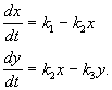
The most interesting results on qualitative modeling of the properties of biological systems were obtained using models of two differential equations that allow qualitative research using the method phase plane. Consider a system of two autonomous ordinary differential equations general view
(4.1)
P(x,y), Q(x,y)- continuous functions, defined in some area G Euclidean plane ( x,y ‑ Cartesian coordinates) and having in this region continuous derivatives of order not lower than the first.
Region G can be either unlimited or limited. If the variables x, y have a specific biological meaning (concentrations of substances, numbers of species) most often the area G represents the positive quadrant of the right half-plane:
0 £ x< ¥ ,0 £ y< ¥ .
Concentrations of substances or numbers of species can also be limited from above by the volume of the vessel or the area of the habitat. Then the range of variables has the form:
0 £ x< x 0 , 0 £ y< y 0 .
Variables x, y change in time in accordance with the system of equations (4.1), so that each state of the system corresponds to a pair of variable values ( x, y).
|
|

 |
Conversely, each pair of variables ( x, y) corresponds to a certain state of the system.
Consider a plane with coordinate axes on which the values of the variables are plotted x,y. Every point M this plane corresponds to a certain state of the system. This plane is called the phase plane and represents the totality of all states of the system. The point M(x,y) is called the representing or representing point.
Let at the initial moment of time t=t 0 coordinates of the representing point M 0 (x(t 0), y(t 0)). At every next moment in time t the representing point will shift in accordance with changes in the values of the variables x(t), y(t). Collection of points M(x(t), y(t)) on the phase plane, the position of which corresponds to the states of the system in the process of changing variables over time x(t), y(t) according to equations (4.1), is called phase trajectory.
The set of phase trajectories for different initial values of the variables gives an easily visible “portrait” of the system. Construction phase portrait allows you to draw conclusions about the nature of changes in variables x, y without knowledge of analytical solutions of the original system of equations(4.1).
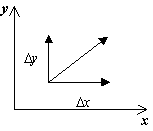
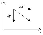
To depict a phase portrait, it is necessary to construct a vector field of directions of system trajectories at each point of the phase plane. Setting the incrementD t>0,we get the corresponding increments D x And D y from expressions:
D x=P(x,y)D t,
D y=Q(x,y)D t.
Vector direction dy/dx at point ( x, y) depends on the sign of the functions P(x, y), Q(x, y) and can be given by a table:
|
P(x,y)>0,Q(x,y)>0 |
|
|
P(x,y)<0,Q(x,y)<0 |
|
|
P(x,y)>0,Q(x,y)<0 |
|
|
P(x,y)<0,Q(x,y)>0 |
|


.(4.2)
Solution to this equation y = y(x, c), or implicitly F(x,y)=c, Where With– constant of integration, gives the family of integral curves of equation (4.2) - phase trajectories system (4.1) on the plane x, y.
Isocline method
To construct a phase portrait they use isocline method - lines are drawn on the phase plane that intersect the integral curves at one specific angle. The isocline equation can be easily obtained from (4.2). Let's put
Where A– a certain constant value. Meaning A represents the tangent of the angle of inclination of the tangent to the phase trajectory and can take values from –¥ to + ¥ . Substituting instead dy/dx in (4.2) the quantity A we obtain the isocline equation:
.(4.3)
Equation (4.3) defines at each point of the plane a unique tangent to the corresponding integral curve, with the exception of the point where P(x,y)= 0, Q (x,y) = 0 , in which the direction of the tangent becomes uncertain, since the value of the derivative becomes uncertain:
![]() .
.
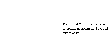
This point is the intersection point of all isoclines - special point. In it, the time derivatives of the variables simultaneously vanish x And y.
![]()
Thus, at a singular point, the rates of change of variables are zero. Consequently, the singular point of the differential equations of phase trajectories (4.2) corresponds to stationary state of the system(4.1), and its coordinates are the stationary values of the variables x, y.
Of particular interest are main isoclines:
dy/dx=0, P(x,y)=0 – isocline of horizontal tangents and
dy/dx=¥ , Q(x,y)=0 – isocline of vertical tangents.
By constructing the main isoclines and finding their intersection point (x,y), whose coordinates satisfy the conditions:
we will thereby find the point of intersection of all isoclines of the phase plane, in which the direction of the tangents to the phase trajectories is uncertain. This - singular point, which corresponds stationary state of the system(Fig. 4.2).
System (4.1) has as many stationary states as there are intersection points of the main isoclines on the phase plane.
Each phase trajectory corresponds to a set of movements of a dynamic system, passing through the same states and differing from each other only in the beginning of the time count.
 |
|

If the conditions of Cauchy’s theorem are satisfied, then through each point in space x, y, t there is only one integral curve. The same is true, due to autonomy, for phase trajectories: a single phase trajectory passes through each point of the phase plane.
Steady State Stability
Let the system be in a state of equilibrium.
Then the representing point is located at one of the singular points of the system, at which, by definition:
![]() .
.
Whether or not a singular point is stable is determined by whether or not the representing point leaves with a small deviation from the stationary state. In relation to a system of two equations, the definition of stability in the languagee, das follows.
The equilibrium state is stable if for any given range of deviations from the equilibrium state (e )you can specify the area d (e ), surrounding the equilibrium state and having the property that no trajectory that begins inside the region d , will never reach the border e . (Fig. 4.4)
 |
|

For a large class of systems - rough systems – the nature of whose behavior does not change with a small change in the form of the equations, information about the type of behavior in the vicinity of a stationary state can be obtained by examining not the original, but a simplified linearized system.
Linear systems.
Consider a system of two linear equations:
![]() .(4.4)
.(4.4)
Here a, b, c, d- constants, x, y- Cartesian coordinates on the phase plane.
We will look for a general solution in the form:
![]() .(4.5)
.(4.5)
Let us substitute these expressions into (4.4) and reduce by e l t:
(4.6)
Algebraic system of equations (4.6) with unknowns A, B has a non-zero solution only if its determinant, composed of coefficients for the unknowns, is equal to zero:
![]() .
.
Expanding this determinant, we obtain the characteristic equation of the system:
.(4.7)
Solving this equation gives the exponent valuesl 1,2 , for which non-zero values are possible for A And B solutions to equation (4.6). These meanings are
![]() .(4.8)
.(4.8)
If the radical expression is negative, thenl 1,2 complex conjugate numbers. Let us assume that both roots of equation (4.7) have nonzero real parts and that there are no multiple roots. Then the general solution of system (4.4) can be represented as a linear combination of exponentials with exponentsl 1 , l 2 :
 (4.9)
(4.9)
To analyze the nature of possible trajectories of the system on the phase plane, we use linear homogeneous coordinate transformation, which will lead the system to canonical form:
![]() ,(4.10)
,(4.10)
allowing a more convenient representation on the phase plane compared to the original system (4.4). Let's introduce new coordinatesξ , η according to the formulas:
(4.1)
From the course of linear algebra it is known that in the case of inequality to zero the real partsl 1 , l 2 the original system (4.4) can always be transformed using transformations (4.11) to the canonical form (4.10) and its behavior on the phase plane can be studiedξ , η . Let us consider the various cases that may present themselves here.
Roots λ 1 , λ 2 – valid and of the same sign
In this case the transformation coefficients are real, we move from the real planex,yto the real plane ξ, η. Dividing the second of equations (4.10) by the first, we obtain:
.(4.12)
Integrating this equation, we find:
Where .(4.13)
Let us agree to understand by λ 2 the root of the characteristic equation with a large modulus, which does not violate the generality of our reasoning. Then, since in the case under consideration the roots λ 1 , λ 2 – valid and of the same sign,a>1 , and we are dealing with integral curves of parabolic type.
All integral curves (except the axis η , which corresponds to ) touch at the origin of the axis ξ, which is also the integral curve of equation (4.11). The origin of coordinates is a special point.
Let us now find out the direction of movement of the representing point along the phase trajectories. If λ 1 , λ 2 are negative, then, as can be seen from equations (4.10), |ξ|, |η| decrease over time. The representing point approaches the origin of coordinates, but never, however, reaches it. Otherwise, this would contradict Cauchy's theorem, which states that only one phase trajectory passes through each point of the phase plane.
Such a special point through which integral curves pass, just like a family of parabolas ![]() passes through the origin and is called a node (Fig. 4.5)
passes through the origin and is called a node (Fig. 4.5)

Equilibrium state of node type at λ 1 , λ 2 < 0 is Lyapunov stable, since the representing point moves along all integral curves towards the origin of coordinates. This stable knot. If λ 1 , λ 2 > 0, then |ξ|, |η| increase over time and the representing point moves away from the origin of coordinates. In this case, the special point– unstable node .
On the phase plane x, y the general qualitative nature of the behavior of integral curves will be preserved, but the tangents to the integral curves will not coincide with the coordinate axes. The angle of inclination of these tangents will be determined by the ratio of the coefficients α , β , γ , δ in equations (4.11).
Roots λ 1 , λ 2 – are valid and of different signs.
Convert from coordinates x,y to coordinates ξ, η again real. The equations for the canonical variables again have the form (4.10), but now the signs of λ 1 , λ 2 are different. The equation of phase trajectories has the form:
Where ,(4.14)
Integrating (4.14), we find
(4.15)
This the equation defines a family of curves of hyperbolic type, where both coordinate axes– asymptotes (at a=1 we would have a family of equilateral hyperbolas). The coordinate axes in this case are also integral curves– these will be the only integral curves passing through the origin. Eachof which consists of three phase trajectories: of two movements to a state of equilibrium (or from a state of equilibrium) and from a state of equilibrium. All other integral curves– are hyperbolas that do not pass through the origin (Fig. 4.6) This special point is called "saddle ». Level lines near a mountain saddle behave similarly to phase trajectories in the vicinity of a saddle.

Let us consider the nature of the movement of the representing point along phase trajectories near the equilibrium state. Let, for example,λ 1 >0 , λ 2<0 . Then the representing point placed on the axis ξ , will move away from the origin, and placed on the axis η – will indefinitely approach the origin of coordinates, without reaching it in a finite time. Wherever the representing point is at the initial moment (with the exception of the singular point and points on the asymptote η =0), it will eventually move away from the equilibrium state, even if it initially moves along one of the integral curves towards the singular point.
It's obvious that a singular point such as a saddle is always unstable . Only under specially selected initial conditions at the asymptoteη =0 the system will approach a state of equilibrium. However, this does not contradict the statement about the instability of the system. If we count, that all initial states of the system on the phase plane are equally probable, then the probability of such an initial state that corresponds to movement in the direction To singular point is equal to zero. Therefore, any real movement will remove the system from the state of equilibrium.Going back to the coordinatesx,y,we will get the same qualitative picture of the nature of the movement of trajectories around the origin of coordinates.
The boundary between the considered cases of a node and a saddle is the case When one of the characteristic indicators, for example λ 1 , vanishes, which occurs when the determinant of the system- expression ad-bc=0(see formula 4.8 ). In this case, the coefficients of the right-hand sides of equations (4.4) are proportional to each other:
and the system has as its equilibrium states all points of the line:
The remaining integral curves are a family of parallel straight lines with an angular coefficient , along which the representing points either approach the equilibrium state or move away from it, depending on the sign of the second root of the characteristic equation λ 2 = a+d.(Fig.4. 7 ) In this case, the coordinates of the equilibrium state depend on the initial value of the variables.

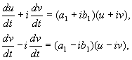
Roots λ 1 , λ 2 – complexconjugate
In this case, for realx And y we will have complex conjugates ξ , η (4.10) . However, by introducing another intermediate transformation, it is also possible in this case to reduce the consideration to a real linear homogeneous transformation. Let's put:
![]() (4.16)
(4.16)
Where a,b, And u,v – actual values. It can be shown that the transformation fromx,y To u,v is, under our assumptions, real, linear, homogeneous with a determinant different from zero. By virtue of the equations(4.10, 4.16) we have:
where
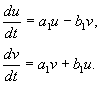 (4.17)
Dividing the second of the equations by the first, we get:
![]()
which is easier to integrate, if we go to the polar coordinate system (r, φ ) . After substitution we get from where:
.(4.18)
Thus, on the phase planeu, vwe are dealing with a family of logarithmic spirals, each of which hasasymptotic point at the origin.A singular point, which is the asymptotic point of all integral curves that have the form of spirals, nested in eachfriend, it's called focus ( Fig.4.8 ) .

Let us consider the nature of the movement of the representing point along phase trajectories. Multiplying the first of equations (4.17) byu, and the second on v and adding, we get:
Where
Let a 1 < 0 (a 1 = Reλ ) . The representing point then continuously approaches the origin of coordinates without reaching it at a finite time. This means that the phase trajectories are twisting spirals and correspond to damped oscillations variables. This - steady focus .
In the case of a stable focus, as in the case of a stable node, not only the Lyapunov condition is satisfied, but also a more stringent requirement. Namely, for any initial deviations, the system will, over time, return as close as desired to the equilibrium position. Such stability, in which the initial deviations not only do not increase, but decay, tending to zero, is called absolute stability .
If in the formula (4.18) a 1 >0 , then the representing point moves away from the origin, and we are dealing with unstable focus . When moving from a planeu,vto the phase planex, ythe spirals will also remain spirals, but will be deformed.
Let us now consider the case whena 1
=0
. Phase trajectories on the planeu, vthere will be circles ![]() which on the planex,ycorrespond to ellipses:
which on the planex,ycorrespond to ellipses:
Thus, whena 1=0 through a special pointx= 0, y= 0 no integral curve passes through. Such an isolated singular point, near which the integral curves are closed curves, in particular, ellipses embedded in each other and enclosing the singular point, is called a center.
Thus, six types of equilibrium states are possible, depending on the nature of the roots of the characteristic equation (4.7). View of phase trajectories on a plane x, y for these six cases is shown in Fig. 4.9.

Rice. 4.9.Types of phase portraits in the vicinity of a stationary state for a system of linear equations (4.4).
The five types of equilibrium states are rough; their character does not change with sufficiently small changes in the right-hand sides of equations (4.4). In this case, changes not only in the right-hand sides, but also in their first-order derivatives should be small. The sixth state of balance – the center – is not rough. With small changes in the parameters of the right side of the equations, it becomes a stable or unstable focus.
Bifurcation diagram
Let us introduce the following notation:
 .
(4.11)
.
(4.11)
Then the characteristic equation will be written as:
![]() .
(4.12)
.
(4.12)
Consider a plane with rectangular Cartesian coordinates s , D and mark on it the areas corresponding to one or another type of equilibrium state, which is determined by the nature of the roots of the characteristic equation
![]() .(4.13)
.(4.13)
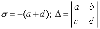
The condition for the stability of the equilibrium state will be the presence of a negative real part of yl 1 and l 2 . A necessary and sufficient condition for this is the fulfillment of the inequalitiess > 0, D > 0 . In diagram (4.15), this condition corresponds to points located in the first quarter of the parameter plane. A singular point will be a focus ifl 1 and l 2 complex. This condition corresponds to those points of the plane for which , those. points between two branches of a parabolas 2 = 4 D. Axle points s = 0, D>0, correspond to equilibrium states of the center type. Likewise,l 1 and l 2 - are valid, but of different signs, i.e. a singular point will be a saddle if D<0, etc. As a result, we will get a diagram of the partition of the parameter plane s, D, into areas corresponding to different types of equilibrium states.

Rice. 4.10. Bifurcation diagram
for a system of linear equations 4.4
If the coefficients of the linear system a, b, c, d depend on a certain parameter, then when this parameter changes, the values will also changes , D . When crossing the boundaries, the character of the phase portrait changes qualitatively. Therefore, such boundaries are called bifurcation boundaries - on opposite sides of the boundary, the system has two topologically different phase portraits and, accordingly, two different types of behavior.
The diagram shows how such changes can occur. If we exclude special cases - the origin of coordinates - then it is easy to see that the saddle can transform into a node, stable or unstable when crossing the ordinate axis. A stable knot can go either into a saddle or into a stable focus, etc. Note that the transitions stable node - stable focus and unstable node - unstable focus are not bifurcations, since the topology of the phase space does not change. We'll talk more about phase space topology and bifurcation transitions in Lecture 6.
During bifurcation transitions, the nature of the stability of a singular point changes. For example, a stable focus through the center can turn into an unstable focus. This bifurcation is called Andronov-Hopf bifurcation by the names of the scientists who studied it. During this bifurcation in nonlinear systems, a limit cycle is born, and the system becomes self-oscillating (see Lecture 8).
Example. Linear chemical reaction system
Substance X flows from outside at a constant speed, turns into substance Y and at a speed proportional to the concentration of the substance Y, is removed from the sphere of reaction. All reactions are of first order, with the exception of the influx of substance from the outside, which is of zero order. The reaction scheme looks like:
(4.14)
and is described by the system of equations:
 (4.15)
We obtain stationary concentrations by equating the right-hand sides to zero:
![]() .(4.16)
.(4.16)
Let us consider the phase portrait of the system. Let us divide the second equation of system (4.16) by the first. We get:
![]() .(4.17)
.(4.17)
Equation (4.17) determines the behavior of variables on the phase plane. Let us construct a phase portrait of this system. First, let's draw the main isoclines on the phase plane. Equation of isocline of vertical tangents:
![]()
Equation of isocline of horizontal tangents:
![]()
The singular point (stationary state) lies at the intersection of the main isoclines.
Now let’s determine at what angle the coordinate axes intersect with the integral curves.
If x= 0, then .
Thus, the tangent of the tangent to the integral curves y=y(x), intersecting the ordinate axis x=0, is negative in the upper half-plane (remember that the variables x, y have concentration values, and therefore we are only interested in the upper right quadrant of the phase plane). In this case, the tangent of the tangent angle increases with distance from the origin.
Consider the axis y= 0. At the point where this axis intersects the integral curves, they are described by the equation
At the tangent of the slope of the integral curves crossing the abscissa axis is positive and increases from zero to infinity with increasing x.
At .
Then, with a further increase, the tangent of the angle of inclination decreases in absolute value, remaining negative and tends to -1 at x ® ¥ . Knowing the direction of the tangents to the integral curves on the main isoclines and on the coordinate axes, it is easy to construct the entire picture of phase trajectories.
 |
|

Let us establish the nature of the stability of the singular point using the Lyapunov method. The characteristic determinant of the system has the form:
![]() .
.
Expanding the determinant, we obtain the characteristic equation of the system: , i.e. The roots of the characteristic equation are both negative. Consequently, the stationary state of the system is a stable node. In this case, the concentration of the substance X tends to a stationary state always monotonically, the concentration of substance Y can pass through min or max. Oscillatory modes are impossible in such a system.
Singular point in mathematics. 1) A singular point of a curve defined by the equation F ( x, y) = 0, - point M 0 ( x 0 , y 0), in which both partial derivatives of the function F ( x, y) go to zero: If not all second partial derivatives of the function F ( x, y) at the point M 0 are equal to zero, then the O. t. is called double. If, along with the first derivatives vanishing at the point M0, all the second derivatives, but not all the third derivatives, vanish, then the equation is called triple, etc. When studying the structure of a curve near a double O.t., the sign of the expression plays an important role If Δ > 0, then the open space is called isolated; for example, at the curve y 2 - x 4 + 4x 2= 0 the origin of coordinates is an isolated O. t. (see. rice. 1
). If Δ x 2 + y 2 + a 2) 2 - 4a 2 x 2 - a 4= 0 the origin of coordinates is the nodal O. t. (see. rice. 2
). If Δ = 0, then the general point of the curve is either isolated or is characterized by the fact that different branches of the curve have a common tangent at this point, for example: a) cusp point of the 1st kind - different branches of the curve are located on opposite sides of the common one tangent and form a point, like a curve y 2 - x 3= 0 (see rice. 3
, a); b) cusp point of the 2nd kind - different branches of the curve are located on one side of the common tangent, like a curve
(y - x 2)2 - x 5= 0 (see rice. 3
, b); c) self-touch point (for a curve y 2 - x 4= 0 the origin is the point of self-touch; (cm. rice. 3
, V). Along with the indicated O. t. there are many other O. t. with special names; for example, the asymptotic point is the vertex of a spiral with an infinite number of turns (see. rice. 4
), termination point, corner point, etc. 2) A singular point of a differential equation is the point at which both the numerator and the denominator of the right side of the differential equation simultaneously vanish (See Differential equations) where P and Q are continuously differentiable functions. Assuming the O. t. is located at the origin of coordinates and using the Taylor formula (See Taylor formula), we can represent equation (1) in the form where P 1 ( x, y) and Q 1 ( x, y) - infinitesimal with respect to Namely, if λ 1 ≠ λ 2 and λ 1 λ 2 > 0 or λ 1 = λ 2, then the O. t. is a node; all integral curves passing through points of a sufficiently small neighborhood of a node enter into it. If λ 1 ≠ λ 2 and λ 1 λ 2 i β, α ≠ 0 and β ≠ 0, then the general point is a focus; all integral curves passing through points in a sufficiently small neighborhood of the focus represent spirals with an infinite number of turns in any arbitrarily small neighborhood of the focus. If, finally, λ 1,2 = ± iβ, β ≠ 0, then the character of the O. t. is not determined by linear terms alone in the expansions of P ( x, y) and Q ( x, y), as was the case in all of the above cases; here O. t. can be a focus or center, or it can have more complex nature. In the neighborhood of the center, all integral curves are closed and contain the center inside themselves. So, for example, the point (0, 0) is a node for the equations at" = 2u/x(λ 1 = 1, λ 2 = 2; see rice. 5
, a) and y" = u/x(λ 1 = λ 2 = 1; see rice. 5
, b), saddle for the equation y" = -y/x(λ 1 = -1, λ 2 = 1 ; cm. rice. 6
), the focus for the equation y" =(x + y) /
(x - y) (λ 1 = 1 - i, λ 2 = 1 + i; cm. rice. 7
) and the center for the equation y" = -x/y(λ 1 = -i, λ 2 = i; cm. rice. 8
). If x, y) and Q ( x, y) analytical, neighborhood O. t. higher order can be divided into regions: D 1 - filled with integral curves, both ends included in the O. t. (elliptic regions), D 2 - filled with integral curves, one end included in the O. t. (parabolic regions), and D 3 - regions , bounded by two integral curves included in the general theory, between which integral curves of the hyperbola type (hyperbolic regions) are located (see rice. 9
). If there are no integral curves included in a general point, then the general point is called a point of stable type. A neighborhood of a stable oscillator consists of closed integral curves containing an osmosis within itself, between which there are spirals (see Fig. rice. 10
). The study of differential equations, that is, essentially the study of the behavior of families of integral curves in the neighborhood of differential equations, constitutes one of the branches of the qualitative theory of differential equations and plays an important role in applications, in particular in questions of stability of motion (works of A. M. Lyapunov, A. Poincaré, etc.). 3) A singular point of a single-valued analytic function is the point at which the analyticity of the function is violated (see Analytical functions). If there is a neighborhood of O. t. a, free from other O. t., then point A called isolated O. t. If A- an isolated general theory and there exists a finite a is called a removable general theory. By appropriately changing the definition of a function at a point a (or redefining it at this point, if the function at it is not defined at all), namely, by assuming f(a)= b, it is possible to achieve that a will become an ordinary point of the corrected function. For example, dot z= 0 is a removable O. t. for the function f 1 ( z) = f(z), If z≠ 0, and f 1 (0), = 1, dot z= 0 is an ordinary point [ f 1 (z) is analytic at the point z= 0]. If A- an isolated O. t. and a is called a pole or an inessentially singular point of a function f(z), if the Laurent series) functions f(z) in the vicinity of an isolated O. t. does not contain negative powers z - a, If A- removable O. t., contains a finite number of negative degrees z - a, If A- pole (in this case the order of the pole R is defined as highest degree a is an essentially singular point. For example, for the function dot z= 0 is the pole of order R, for function dot z= 0 is an essentially singular point. On the boundary of the circle of convergence of a power series there must be at least one O.t. of the function represented within this circle by the data power series. All boundary points of the domain of existence of a unique analytic function (natural boundary) are the boundaries of this function. Thus, all points of the unit circle | z| = 1 are special to the function For a multi-valued analytic function, the concept of “O. T." more difficult. In addition to the O. t., in individual sheets of the Riemann surface of a function (that is, the O. t. of single-valued analytic elements), each branch point is also the O. t. of the function. Isolated branch points of a Riemann surface (that is, such branch points that in some neighborhood of them there are no other O. t. functions in any leaf) are classified as follows. If a is an isolated branch point of finite order and there is a finite a, it is called a critical pole. If A- an isolated branch point of infinite order and a is called a transcendental O.t. All other isolated branch points are called critical essentially singular points. Examples: dot z= 0 is the ordinary critical point of the function f ( z) = log z and the critical essentially singular point of the function f (z) = sin ln z. Every general theory, except a removable one, is an obstacle to analytical continuation, that is, analytical continuation along a curve passing through an irreducible general problem is impossible. Big Soviet encyclopedia. - M.: Soviet Encyclopedia.
1969-1978
.

![]()
![]()
 p = 2, 3, …)


See what a “Singular point” is in other dictionaries:
Points here. See also singular point ( differential equations). A feature or singularity in mathematics is a point at which a mathematical object (usually a function) is undefined or has irregular behavior (for example, a point at which ... ... Wikipedia
An analytic function is a point at which the conditions of analyticity are violated. If the analytic function f(z) is given in a certain neighborhood of the point z0 everywhere... Physical encyclopedia
An analytic function is the point at which the analyticity of the function is violated... Big Encyclopedic Dictionary
singular point- - [Ya.N.Luginsky, M.S.Fezi Zhilinskaya, Yu.S.Kabirov. English-Russian dictionary of electrical engineering and power engineering, Moscow, 1999] Topics of electrical engineering, basic concepts EN singular point ... Technical Translator's Guide
1) An analytic function f(z) is an obstacle to the analytic continuation of an element of a function f(z) of a complex variable z along any path on the plane of this variable. Let the analytic function f(z) be defined by some... ... Mathematical Encyclopedia
Analytical function, the point at which the analyticity of the function is violated. * * * SINGLE POINT SINGLE POINT of an analytical function, the point at which the analyticity of the function is violated... encyclopedic Dictionary
singular point- ypatingasis taškas statusas T sritis automatika atitikmenys: engl. singular point vok. singulärer Punkt, m rus. singular point, f pranc. point particulier, m; point singulier, m … Automatikos terminų žodynas
singular point- ypatingasis taškas statusas T sritis fizika atitikmenys: engl. singular point vok. singulärer Punkt, m rus. singular point, f pranc. point singulier, m … Fizikos terminų žodynas
Basic concepts and definitions:
The zero of the analytic function f(z) is the point “a” for which f(a)=0.
A zero of order “n” of a function f(z) is a point “a” if fn(a)¹0.
A singular point “a” is called an isolated singular point of a function f(z) if there is a neighborhood of this point in which there are no singular points other than “a”.
There are three types of isolated singular points: .
1 removable singular points;
3 essentially singular points.
The type of singular point can be determined based on the behavior of a given function at the found singular point, as well as from the form of the Laurent series obtained for the function in the neighborhood of the found singular point.
Determining the type of a singular point by the behavior of the function at it.
1. Removable singular points.
An isolated singular point a of a function f(z) is called removable if there is a finite limit.
2.Poles.
An isolated singular point a of a function f(z) is called a pole if ![]() .
.
3. Essentially singular points.
An isolated singular point a of a function f(z) is called an essentially singular point if neither finite nor infinite exists.
The following relationship exists between the zeros and poles of the function.
In order for point a to be a pole of order n of the function f(Z), it is necessary and sufficient that this point be a zero of order n for the function .
If n=1 the pole is called simple.
Definition: An isolated singular point of unambiguous nature is called:
a) removable if the main part of the decomposition is missing;
b) a pole, if the main part contains a finite number of terms;
c) an essentially singular point if the main part contains an infinite number of terms.
a) Thus, in the neighborhood of a removable singular point, the expansion has the form:
it expresses the function at all points of the circle |z-a| At the center z=a the equality is not true, because the function at z=a has a discontinuity, and the right side is continuous. If the value of the function in the center is changed, taking it equal to the value of the right side, then the gap will be eliminated - hence the name - removable. b) In the neighborhood of a pole of order m, the Laurent series expansion has the form: c) In the vicinity of a simple pole Deductions and formulas for calculating them. The residue of an analytic function f(z) at an isolated singular point z 0 is a complex number equal to the value of the integral The residue of the function f(z) at an isolated singular point z 0 is denoted by the symbol Res f(z 0) or Res (f(z); z 0). Thus, Res f(z 0)= If we put n=-1 in formula (22.15.1), we get: C -1 = or Res f(z 0)= C -1 , those. the residue of the function f(z) with respect to the singular point z 0 is equal to the coefficient of the first term with a negative exponent in the expansion of the function f(z) in the Laurent series. Calculation of deductions. Regular or removable singular points. Obviously, if z=z 0 is a regular or removable singular point of the function f(z), then Res f(z 0)=0 (the Laurent expansion in these cases lacks the main part, so c-1=0). Pole. Let the point z 0 be a simple pole of the function f(z). Then the Laurent series for the function f(z) in the vicinity of the point z 0 has the form: From here Therefore, passing in this equality to the limit at z --z 0, we obtain Res f(z0)= Essentially special point. If the point z 0 is an essentially singular point of the function f(z), then to calculate the residue of the function at this point, the coefficient c-1 in the Laurent series expansion of the function is usually directly determined. Classification of events. Sum, product of events, their properties, graphical representation. Events are divided into: 1. Random 2. Reliable 3. Impossible Reliable is an event that necessarily occurs under given conditions (night follows morning). A random event is an event that may or may not happen (passing an exam). An impossible event is an event that will not occur under given conditions (getting a green pencil out of a box with only red ones). Let zq is the singular point of the function /(r), t.s. f(z) but is analytic at this point (in particular, it may not be defined at it). If there is such a punctured neighborhood of the point zq (i.e. the set O z - zq f(z) is aialitic, then zo called isolated singular point functions f(z). This definition remains the same in the case of zn = oo, if the iodine is pierced by the vicinity of the point zq = oo understand set z> I -
the exterior of a circle with its center at the origin. In other words, a special point zq is said to be isolated if there is a neighborhood of this point in which the ist of other singular points other than zq. Throughout what follows we consider only singular points of a unique character (the function f(z) assumed to be unambiguous). Depending on the behavior of the function f(z) at z -> zq There are three types of singular points. Isolated singular point zq functions f(z) called: 1) removable singular point, if there is a finite limit 2) pole, if there is a limit 3) essentially a special point, If f(z) has neither a finite nor an infinite limit at z-> zq. Example 26.1. Let us show that all three types of singular points are realized. Let's consider f(z)= Point zq = 0 is isolated special point of this function. Using formula (22.12), we obtain the expansion from which it follows that there exists lim fi(z)= 1. Therefore zq = 0 is is a removable singular point of the function fi(z). Function f‘j(z) =---has a pole at a point zo= 1 because 2
r“ X Let us now consider the function )з(z)= e 1 ^ r and show that zo = O is an essentially singular point of this function. When striving z to zero along the real axis the left and right limits of the function /z (z) different: lim With 1 / 1
=
0, lim s 1 /* = os. This implies, x->0-0 x->0+O What f:i(z) has neither finite nor infinite limit at 2 ->
Oh, that is. zq = O is an essentially singular point of this function. (Note that as the point tends z - iy to zero along the imaginary axis function has no limit at all.) There are, of course, non-isolated singular points. For example. the function has poles at points z n = -, P= ±1, ±2,... Hence, Zq = 0 is a non-isolated singular point of this function: in any (no matter how small) neighborhood of this point there are other singular points g p.
Let zo- finite isolated singular point of a function f(z). Then f(z) is similar in some punctured neighborhood of the 0 Zo point zo this neighborhood can be considered as a ring with internal radius r = 0. By Theorem 25.1, in the neighborhood under consideration the function f(z) can be expanded into a Laurent series (25.2). We will show that the behavior of the function at 2 -> zq (i.e. the type of singular point zo) depends on the type of the main part of the expansion (25.2); This circumstance explains the origin of the term “main part”. Theorem 2G.2. An isolated singular point zo of a function f(z) is removable if and only if the Lorapov expansion in a punctured neighborhood of this point has oid those. consists of only the correct part, and all coefficients of the main part are equal to the bullet. Proof. 1. Let zo- removable singular point. Let us prove that the Laurent expansion of the function f(z) has the form (26.1). Since the special point zo removable, then there is a finite limit lim f(z) = A. Hence, f(z) is bounded in some punctured neighborhood of the 0 z - zq point zo, those. )(z) for everyone z from this vicinity. Let's take any R. U р /?|, and use formulas (25.3) for the coefficients of the Laurent series: For the coefficients of the main part of the expansion n =- 1,-2,... For such values P we have p~ p-e 0 at R-> 0. Since the value R can be chosen arbitrarily small, then Mr~" can be as small as desired. Since |s t,| ^ Mr~p and c„ do not depend on p, then c„ = 0 at And= - 1, -2,..., which is what needed to be proven. 2. Let us now assume that the Laurent expansion has the form (26.1). The series (26.1) is a power series and. therefore, it converges not only in the punctured area, but also in the entire vicinity z-zq including the point zo; its amount S(z) is analytic at z and S(z) = )(z) at 0 z - zo R. Therefore there is a finite limit lim )(z)= Pt 5(g) = 5(th) - Therefore, the singular point zq Z->Zo Z-*Zo removable. The theorem has been proven. Comment. From the proof of the theorem it follows that in a punctured neighborhood 0 z - zo of a removable singular point the function f(z) coincides with the function 5(r), which is analytic in the entire neighborhood z - zo. Therefore, if we set /(th) = S(zq), then, without changing the function values f(z) at any points of the punctured neighborhood, we will make this function analytic in Go, i.e. Let’s “eliminate” the feature. This explains the term “removable feature”. It is natural to consider such points to be regular, and not singular points of the function f(z).
Consider, for example, the function In example 26.1 it was shown that Pm Nr) = 1. i.e. singular point zq = 0 removable. Setting /i(0) = 1, we thereby eliminate the singularity and obtain a function that is analytic at the point zq = 0 (and throughout the C plane). Let us now characterize the poles in terms of Laurent expansions. Theorem 26.3. An isolated singular point Zo of a function f(z) is a pole if and only if, when the main part of the Laurent expansion with center Zq has only a finite number of distinct from zero coefficients with n: Proof. 1. Let zq - pole, i.e. lim/( z) = oo. Let us prove that the Laurent expansion of the function f(z) has the form (2G.2). Since lim f(z)= oo. then there is a punctured neighborhood of the point ki zq. wherein f(z) is analytic and has no zeros. Then the function g(z) = 1 /f(z) will also be analytic in this punctured neighborhood, and lim g(z)= 0. Therefore, Zo is removable *-? *0 singular point of the function g(z). Let's define g(z) at the point zo, putting g(zo)=
0. Then g(z) will become analytic in the entire neighborhood of the (not pierced) point z 0 , and z 0 will be its isolated zero. Let us denote by N multiplicity (order) of this zero. As was shown in §23, in the neighborhood of the point zq function g(z) can be represented in the form (see (23.2)) and (z$) f 0 and y>(z) is analytic in some neighborhood of the point zo- Because ip(z) continuous at a point zo And g>(zo) Ф 0" then ip(z) has no zeros in some neighborhood of this point. Therefore function 1 /-p(z) will also be analytic in this neighborhood and, therefore, expands in it in a Taylor series: Opening the brackets and changing the designations of the coefficients, we write the last expansion in the form where c_jv = 1>o f 0. Thus, the main part of the Laurent expansion of the function /(r) contains only a finite number of terms; we have arrived at the desired equality (26.2). 2. Let in the punctured neighborhood of points th function )(z) is represented by the Laurent expansion (26.2) (for a more detailed form, see (26.3)), the main part of which contains only a finite number of terms, and With- d" f 0. It is necessary to prove that Zq - function pole f(z). Multiplying equality (26.3) by (G - G o) iV , we get the function The series in (26.4) is a power series that converges to an analytic function not only in the punctured point, but also in the entire neighborhood of the point Zq. Therefore the function h(z) will become analytic in this neighborhood if we further define it in go by putting h(zo)= s_dg f 0. Then Thus, the point th is a pole, and Theorem 26.3 is proven. Multiplicity (order) of zero function g(z)= 1//(g) is called pole order th function /(r). If N- the order of the pole of th, then g(z)= (g - Zo) N ip(z), and (go) F 0, and, as shown in the first part of the proof of Theorem 26.3, the expansion of the function /(r) has the form (26.3), where c_/v f 0. Conversely, if /(r) is expanded into the series (26.3) and e-i F 0, then t.s. N- order of the pole of the function /(r). Thus, pole order of the zq function/(G) equal to the number of the highest nonzero coefficient of the main part of the Laurent expansion in the punctured neighborhood of the point zq(i.e. equal to this number N, what s_dg f 0 and Sp= 0 at P > N). Let us prove the following statement, which is convenient for applications. Corollary 26.4. The point zq is a pole of order N of the fiction/(G) then and only when/(G) representable in the form where h(z) is an analytical function in the vicinity of the point th and h(zo) f 0. Proof. Function cp(z) = l/h(z) is analytic in some neighborhood of the point h. The condition of Corollary 26.4 is equivalent to the following: That's why zq -
zero multiplicity N functions g(z). and therefore the pole of multiplicity N functions /(2). II Example 26.5. Find isolated singular points of a function Solution: The points at which (z 2
+ 1 )(z+ Z) 2 = 0. If z 2
L- 1 = 0, then 2 = ±g If (z 4- 3) 2 = 0, then z= -3. Therefore the function has three singular points z= g, 22 = -g, Z3
=
- 3. Consider z: G - first order pole (we used Corollary 26.4). It can be proven in a similar way that 22 = -i also a pole of first order. For 2z we have: Let us move on to consider essentially singular points. Theorem 26.6. An isolated singular point zq of a function f(z) is essentially singular if and only if the principal part of the Laurent expansion with center zq has infinitely many distinct from. zero, coefficients from p. Proof. Theorem 26.6 follows directly from Theorems 26.2 and 26.3. Indeed, if the point zq is essentially special, then the main part of the Laurent expansion cannot be absent or contain a finite number of terms (otherwise the point Zq will be either removable or a pole). Therefore, the number of terms in the main part must be infinite. Conversely, if the main part contains infinitely many terms, then Zq can be neither a removable point nor a pole. It follows that this point is essentially special. According to the definition, an essentially singular point is characterized by the fact that the function /(2) has neither a finite nor an infinite limit for z ->zq. A more complete idea of how irregular the behavior of a function is in the neighborhood of an essentially singular point is given by the following theorem. Theorem 26.7 (Sokhotsky's theorem). If zq is essential to persons, the point of the function f(z), then for any complex number L, including A = oh, there is a sequence of points z n such that z n -> zo and lim f(zn) = A. p->os Proof. Let us first consider the case A = oo. In the first part of the proof of Theorem 2G.2 we established that if f(z) is bounded in some punctured neighborhood of the point r, then all the coefficients c", n = - 1,- 2,... of the main part are equal to zero (and, therefore, the singularity in go is removable). Since by condition th is an essential singular point, then in any punctured neighborhood of the point th the function f(r) is unbounded. Let us take some strong neighborhood 0 Z such that f(zi) > 1 (if |/(r)| z - zo I/2 there is a point z-2
, in which |/(yy)| > 2, etc.: in the punctured neighborhood O 71.
It is obvious that r„ -e go and lim /(r“) = oo. Thus, in the case A = oo, Theorem 26.7 proven. Let it now A f oo. Let us first assume that there is a punctured neighborhood 0 = -yy----
will be analytical in this punctured neighborhood and, consequently, /(G) - A Consequently, go is an isolated singular point of the function Φ(r). We'll show you. that r is an essentially singular point of Φ(r). This may not be true. Then there is a limit lim Ф(r), finite or infinite. For a while /(r) = A + , then there is also Hsh /(r), which contradicts the condition F(g) ~ :-*z 0 I see the theorem. Thus, r0 is an essentially singular point of the function Φ(r). According to what was proved above, there is a sequence of points r n such that r n th and lim Ф(r n) = oo. From here We have proved the required statement under the assumption that /(r) F A in some punctured neighborhood of the point go- Let us now assume that this is false, i.e. in any arbitrarily small punctured neighborhood of the point th there is such a point G", that /(r") = L. Then for any P in the punctured neighborhood 0 f(z u) = А. Thus, the desired statement is true P-yuo in all cases, and Theorem 26.7 is proven. According to Theorem 26.7 (Sokhotsky), in any (arbitrarily small) punctured neighborhood of an essentially singular point, the function /(r) takes on values arbitrarily close to any number from the extended complex plane C. To study isolated singular points, the already known Taylor expansions of basic elementary functions are often useful. Example 2G.8. Determine the type of singular point zq = 0 for the function Solved and e. Let us expand the numerator and denominator into a Taylor series in powers of g. Substituting in (22.11) 3 z instead of r and subtracting 1, we get Using (22.12), we obtain the expansion of the denominator: The series in these expansions converge in the entire complex plane €. We have and /2(2) are anaritic in a neighborhood of the point zo = 0 (and even in the entire plane) and /2(20) F 0, then h(z) is also analytic in some neighborhood of the point gF 0. According to Corollary 26.4, the point Zo = 0 is the pole of order N=4. II Example 26.9. Find singular points of a function f(z)= sin j - and determine their type. R e in e i e. The function has a single finite singular point zq = 1. At other points from C the function w =--- analytical; hence the function sin w will be analytical. Substituting - instead of r into the expansion of sine (22.12), we get We have obtained an expansion of the function sin into a Laurent series in a punctured neighborhood of the point 2o = 1. Since the resulting expansion contains infinitely many terms with negative powers (r - 1), then zq = 1 is an essentially singular point (in this case, the Laurent expansion consists only of the main part, and the regular part is missing). Note that it was possible to establish the nature of the singularity in this case directly from the definition, without resorting to series expansion. Indeed, there are sequences (r",) and (2") converging to zo= 1, and such that f(z"n)= 1, /(2") = 0 (indicate such sequences yourself). So, f(z) has no limit at z -> 1 and therefore point zq - 1 is essentially special. Let us introduce the concept of Laurent expansion of a function in a neighborhood of a point Zq = 00 and consider the connection between the expansion and the nature of the singularity at this point. Note that the definitions of an isolated singular point and its type (removable, pole, or essentially singular) carry over to the case zq = oc without changes. But Theorems 26.2. 26.3 and 26.6, related to the nature of the Laurent expansions, need to be changed. The point is that members cn(z- 2o) p. P= -1,-2,..., main part, defining the “irregularity” of the function near the end point Zq, as 2 tends to oo, they will behave “correctly” (tend to 0). On the contrary, the members of the correct part with P= 1,2,... will tend to oo; they determine the nature of the feature in Zq = oo. Therefore, the main part of the expansion in the vicinity of oo will consist of terms with positive powers P, and the correct one - with negative ones. Let's introduce a new variable w = 12. Function tv = 1/2, extended so that u(oo) = 0, one-to-one and conformally maps the neighborhood z > R points zq = 00 in the vicinity of |w| wq = 0. If the function f(z) analytics in the punctured neighborhood R z Zq = oc, then the function G(w) = f(l/w) will be analytic in the great neighborhood 0 wo = 0. Since at 2 -> oo there will be w-> 0, then That's why G(w) has at the point wq = 0 is a feature of the same type as f(z) at the point Zq = 00. Let us expand the function G(w) into a Laurent series in a punctured neighborhood of the point wo = 0: The sums on the right side of (26.5) represent the regular and principal parts of the expansion, respectively. Let's move on to the variable z, substituting w = 1/z: Designating P= -A*, 6* = 6_„ = s p and noticing that G(l/z) = f(z), we get The decomposition (2G.G) is called Laurent expansion of the function f(z) in a punctured neighborhood of the point zq= oo. The first sum in (2G.6) is called the right part, and the second sum is main part of this decomposition. Since these sums correspond to the correct and principal parts of expansion (26.5), then analogues of Theorems 26.2, 26.3 and 26.6 are valid for expansion (26.6). Thus, the following theorem will be an analogue of Theorem 26.2. Theorem 26.10. Isolated singular pointZq -
OS (functions/(G) is removable if and only if the Laurent expansion in a punctured neighborhood of this point has the form
t.s. consists of only the correct part. Let us put /(oo) = co. Function defined by series (26.7) converging in the neighborhood z > R point 2o = oc, called analytical at point z o = oo. (Note that this definition is equivalent to the analyticity of the function G(w) at point wo = 0.) Example 26.11. Investigate the singular point zq = oo of the function Since the limit is finite, then zo = oo is a removable singular point of the function /(r). If we put /(oo) = lim J(z)= 0, then f(z) will become analytical tic at the point Zo= os. Let us indicate how to find the corresponding expansion (26.7). Let's move on to the variable w = 1 fz. Substituting z= 1 /?е, we get (the last equality is valid in a punctured neighborhood of the point wо = 0, but we will further define (7(0) = 0). The resulting function has singular points w =±i, w =-1/3, and at the point Wq = 0 is analytic. Unfolding function G(w) by degrees w(as was done in Example 25.7) and substituting into the resulting power series w = 1/z, we can obtain expansion (26.7) of the function f(z).
Theorem 26.3 for the case zo= oo will be rewritten in the following form. Theorem 26.12. Isolated singular point th = os function f(z) is a pole if and only if the principal part of the Laurent expansion (26.6) has only a finite number of nonzero coefficients With": Here the series is the regular part, and the polynomial in brackets is the main part of the expansion. The pole multiplicity in oc is defined as the pole multiplicity wq = 0 functions G(z). It is easy to see that the multiplicity of the pole coincides with the number N in (26.8). Q p | (i 2 + 1)(z+3) 2 Task. Show that the function f(z) =--
-- has in point zo = oo pole of order 3. Theorem 26.6 on an essentially singular point can be rewritten for the case zo= os almost verbatim, and we do not dwell on this in detail. , taken in the positive direction along the circle L with center at point z 0 lying in the domain of analyticity of the function f(z) (i.e. in the ring 0<|z-z0| . (22.15.1)

![]()


 and determine their type.