Three equivalent definitions of a function continuous at a point. continuous function

Theorem. Let the function x=φ(t) continuous at point a, and the function y=f(x) continuous at point b=φ(a). Then the complex function y=f[φ(t)]=F(t) continuous at point a.

Let x=φ(t) and y=f(x) are the simplest elementary functions, and the set of values (x) functions x=φ(t) is the scope of the function y=f(x). As we know, elementary functions are continuous at every point of the task area. Therefore, according to the previous theorem, the complex function y=f(φ(t)), that is, the superposition of two elementary functions, is continuous. For example, the function is continuous at any point x ≠ 0, as a complex function of two elementary functions x=t-1 and y=sin x. Also function y=ln sin x continuous at any point of the intervals (2kπ,(2k+1)π), k ∈ Z (sinx>0).

1. Introduction.

2. Definition of the continuity of a function.

3. Classification of discontinuity points

4. Properties of continuous functions.

5. Economic meaning of continuity.

6. Conclusion.

10.1. Introduction

Every time, assessing the inevitable changes in the world around us over time, we try to analyze the ongoing processes in order to highlight their most significant features. One of the first questions on this path is: how changes that are characteristic of this phenomenon occur - continuously or discretely, i.e. spasmodically. Does the currency depreciate evenly or collapse, is there a gradual evolution or a revolutionary leap? In order to unify the qualitative and quantitative assessments of what is happening, one should abstract from the specific content and study the problem in terms of functional dependence. This allows us to do the theory of limits, which we considered in the last lecture.

10.2. Determining the continuity of a function

The continuity of a function is intuitively related to the fact that its graph is a continuous, nowhere interrupted curve. We draw a graph of such a function without lifting the pen from the paper. If a function is given in a table, then its continuity, strictly speaking, cannot be judged, because for a given step of the table, the behavior of the function in the intervals is not defined.

In reality, with continuity, the following circumstance takes place: if the parameters characterizing the situation a little change then a little the situation will also change. The important thing here is not that the situation will change, but that it will change “a little”.

Let us formulate the concept of continuity in the language of increments. Let some phenomenon be described by a function and a point a belongs to the scope of the function. The difference is called argument increment at the point a, the difference is function increment at the point a.

Definition 10.1.Function continuous at point a if it is defined at this point and an infinitesimal increment of the argument corresponds to an infinitesimal increment of the function :

Example 10.1. Investigate for continuity a function at a point .

Solution. Let's build a graph of the function and mark the increments D on it x and D y(Fig. 10.1).

It can be seen from the graph that the smaller the increment D x, the less D y. Let's show this analytically. The increment of the argument is , then the increment of the function at this point will be equal to

This shows that if , then and :

.

Let us give one more definition of the continuity of a function.

Definition 10.2.The function is called continuous at point a if:

1) it is defined at the point a, and some of its neighborhood;

2) one-sided limits exist and are equal to each other:

;

3) limit of the function at x® a is equal to the value of the function at that point:

.

If at least one of these conditions is violated, then the function is said to undergo gap.

This definition is working for establishing continuity at a point. Following his algorithm and noting the coincidences and discrepancies between the requirements of the definition and a specific example, we can conclude that the function is continuous at a point.

Definition 2 clearly shows the idea of ​​proximity when we introduced the concept of limit. With unlimited approximation of the argument x to limit value a, continuous at the point a function f(x) arbitrarily close to the limiting value f(a).

10.3. Classification of break points

The points at which the conditions for the continuity of a function are violated are called breaking points this function. If a x 0 is the discontinuity point of the function , at least one of the continuity conditions for the function is not satisfied in it. Consider the following example.

1. The function is defined in some neighborhood of the point a, but not defined at the point itself a. For example, the function is not defined at the point a=2, so it undergoes a discontinuity (see Fig. 10.2).

Rice. 10.2 Fig. 10.3

2. The function is defined at a point a and in some neighborhood of it, its one-sided limits exist, but are not equal to each other: , then the function undergoes a discontinuity. For example, the function

is defined at the point , however, when the function experiences a discontinuity (see Fig. 10.3), because

and ().

3. The function is defined at a point a and in some of its neighborhood, there is a limit of the function at , but this limit is not equal to the value of the function at the point a:

.

For example, a function (see Figure 10.4)

Here is the breaking point:

,

All discontinuity points are divided into removable discontinuity points, discontinuity points of the first and second kind.

Definition 10.1. The breaking point is called a point repairable gap , if at this point there are finite limits of the function on the left and on the right, equal to each other:

.

The limit of the function at this point exists, but is not equal to the value of the function at the limit point (if the function is defined at the limit point), or the function at the limit point is not defined.

On fig. 10.4 at the point, the continuity conditions are violated, and the function has a discontinuity. Point (0; 1) on the chart gouged out. However, this gap can be easily eliminated - it is enough to redefine the given function, setting it equal to its limit at this point, i.e. put . Therefore, such gaps are called removable.

Definition 10.2. The breaking point is called discontinuity point of the 1st kind , if at this point there are finite limits of the function on the left and on the right, but they are not equal to each other:

.

At this point, the function is said to experience jump.

On fig. 10.3 the function has a discontinuity of the 1st kind at the point . The limits on the left and right at this point are equal:

and .

The jump of the function at the discontinuity point is equal to .

It is impossible to extend such a function to a continuous one. The graph consists of two half-lines separated by a jump.

Definition 10.3. The breaking point is called breaking point of the 2nd kind if at least one of the function's one-sided limits (left or right) does not exist or is equal to infinity.

In Figure 10.3, the function at a point has a discontinuity of the 2nd kind. The considered function at is infinitely large and has no finite limit either on the right or on the left. Therefore, it is not necessary to speak of continuity at such a point.

Example 10.2. Build a graph and determine the nature of the break points:

Solution. Let's plot the function f(x) (Figure 10.5).

It can be seen from the figure that the original function has three break points: , x 2 = 1,
x 3 = 3. Consider them in order.

Therefore, the point has rupture of the 2nd kind.

a) The function is defined at this point: f(1) = –1.

b) , ,

those. at the point x 2 = 1 available repairable gap. By overriding the value of the function at this point: f(1) = 5, the discontinuity is eliminated and the function becomes continuous at this point.

a) The function is defined at this point: f(3) = 1.

So at the point x 1 = 3 available rupture of the 1st kind. The function at this point experiences a jump equal to D y= –2–1 = –3.

10.4. Properties of continuous functions

Recalling the corresponding properties of limits, we conclude that a function that is the result of arithmetic operations on functions continuous at the same point is also continuous. Note:

1) if the functions and are continuous at a point a, then the functions , and (provided that ) are also continuous at this point;

2) if the function is continuous at a point a and the function is continuous at the point , then the compound function is continuous at the point a and

,

those. the sign of the limit can be placed under the sign of the continuous function.

They say that a function is continuous on some set if it is continuous at every point of that set. The graph of such a function is a continuous line, which is crossed out with one stroke of the pen.

All major elementary functions are continuous at all points where they are defined.

Functions, Continuous on the segment, have a number of important distinguishing properties. Let us formulate theorems expressing some of these properties.

Theorem 10.1 (Weierstrass theorem ). If a function is continuous on a segment, then it reaches its minimum and maximum values ​​on this segment.

Theorem 10.2 (Cauchy's theorem ). If a function is continuous on a segment, then it is on this segment all intermediate values ​​between the smallest and largest values.

The following important property follows from Cauchy's theorem.

Theorem 10.3. If a function is continuous on a segment and takes values ​​of different signs at the ends of the segment, then between a and b there is a point c at which the function vanishes:.

The geometric meaning of this theorem is obvious: if the graph of a continuous function passes from the lower half-plane to the upper one (or vice versa), then at least at one point it will intersect the axis Ox(fig.10.6).

Example 10.3. Approximately calculate the root of the equation

, (i.e. approximately replace) polynomial of the corresponding degree.

This property of continuous functions is very important for practice. For example, very often continuous functions are given by tables (observational or experimental data). Then, using any method, you can replace the table function with a polynomial. In accordance with Theorem 10.3, this can always be done with sufficiently high accuracy. Working with an analytically given function (especially with a polynomial) is much easier.

10.5. The economic meaning of continuity

Most of the functions used in the economy are continuous, and this allows us to make quite significant statements of economic content.

As an illustration, consider the following example.

tax rate N has a graph similar to Fig. 10.7a.

At the ends of the gaps it is discontinuous and these discontinuities are of the first kind. However, the amount of income tax P(Fig. 10.7b) is a continuous function of annual income Q. From this, in particular, it follows that if the annual incomes of two people differ insignificantly, then the difference in the amount of income tax that they must pay should also differ insignificantly. It is interesting that the circumstance is perceived by the vast majority of people as completely natural, over which they do not even think.

10.6. Conclusion

In the end, let's take a little digression.

Here is how to graphically express the sad observation of the ancients:

Sic transit Gloria mundi …

(This is how earthly glory passes …)

End of work -

This topic belongs to:

Function concept

The concept of function.. everything flows and everything changes Heraclitus.. table x x x x y y y y y y y y y

If you need additional material on this topic, or you did not find what you were looking for, we recommend using the search in our database of works:

What will we do with the received material:

If this material turned out to be useful for you, you can save it to your page on social networks:

Definition
function f (x) called continuous at x 0 neighborhood of this point, and if the limit as x tends to x 0 equals the value of the function in x 0 :
.

Using the Cauchy and Heine definitions of the limit of a function, one can give detailed definitions of the continuity of a function at a point .

One can formulate the concept of continuity in terms of increments. To do this, we introduce a new variable, which is called the increment of the variable x at the point. Then the function is continuous at the point if
.
Let's introduce a new function:
.
They call her function increment at point . Then the function is continuous at the point if
.

Continuity definition right (left)
function f (x) called continuous on the right (left) at the point x 0 , if it is defined on some right-handed (left-handed) neighborhood of this point, and if the right (left) limit at the point x 0 equals the value of the function in x 0 :
.

Boundedness theorem for a continuous function
Let the function f (x) continuous at x 0 . Then there exists a neighborhood U (x0) on which the function is limited.

Theorem on the conservation of the sign of a continuous function
Let the function be continuous at the point . And let it have a positive (negative) value at this point:
.
Then there is such a neighborhood of the point on which the function has a positive (negative) value:
at .

Arithmetic properties of continuous functions
Let the functions and be continuous at the point .
Then the functions , and are continuous at the point .
If , then the function is also continuous at the point .

Left and Right Continuity Property
A function is continuous at a point if and only if it is continuous at the right and left.

Proofs of the properties are given on the page "Properties of functions continuous at a point".

Continuity of a complex function

Complex function continuity theorem
Let the function be continuous at the point . And let the function be continuous at the point .
Then the complex function is continuous at the point .

Complex function limit

Theorem on the limit of a continuous function of a function
Let there be a limit of the function at , and it is equal to:
.
Here point t 0 can be finite or at infinity: .
And let the function be continuous at the point .
Then there is a limit of the complex function , and it is equal to:
.

Complex function limit theorem
Let the function have a limit and map the punctured neighborhood of the point onto the punctured neighborhood of the point . Let the function be defined on this neighborhood and have a limit on it.
Here - final or infinitely distant points: . Neighborhoods and their corresponding limits can be either two-sided or one-sided.
Then there is a limit of the complex function and it is equal to:
.

break points

Determining the Break Point
Let the function be defined on some punctured neighborhood of the point . The point is called function break point if one of the two conditions is met:
1) not defined in ;
2) is defined at , but is not at that point.

Determination of the break point of the 1st kind
The point is called breaking point of the first kind, if is a breakpoint and there are finite one-sided limits on the left and on the right:
.

Function jump definition
Jump Δ function at a point is called the difference between the limits on the right and on the left
.

Determining a break point
The point is called break point if there is a limit
,
but the function at the point is either not defined or is not equal to the limit value: .

Thus, a discontinuity point is a discontinuity point of the 1st kind, at which the jump of the function is equal to zero.

Determination of the break point of the 2nd kind
The point is called breaking point of the second kind, if it is not a discontinuity point of the 1st kind. That is, if there is not at least one one-sided limit, or at least one one-sided limit at a point is equal to infinity.

Properties of functions continuous on an interval

Definition of a function continuous on a segment
A function is called continuous on a segment (at ) if it is continuous at all points of the open interval (at ) and at points a and b , respectively.

Weierstrass' first theorem on the boundedness of a function continuous on an interval
If a function is continuous on a segment, then it is bounded on this segment.

Determination of reachability of the maximum (minimum)
The function reaches its maximum (minimum) on the set if there is an argument for which
for all .

Determining the reachability of the upper (lower) bound
A function reaches its upper (lower) bound on the set if there is an argument for which
.

The second theorem of Weierstrass on the maximum and minimum of a continuous function
A function continuous on a segment reaches its upper and lower bounds on it or, which is the same thing, reaches its maximum and minimum on the segment.

Bolzano-Cauchy intermediate value theorem
Let the function be continuous on the interval . And let C be an arbitrary number between the values ​​of the function at the ends of the segment: and . Then there is a point for which
.

Corollary 1
Let the function be continuous on the interval . And let the function values ​​at the ends of the segment have different signs: or . Then there is a point where the value of the function is equal to zero:
.

Consequence 2
Let the function be continuous on the interval . Let it go . Then the function takes on the segment all values ​​from and only these values:
at .

Inverse functions

Definition of the inverse function
Let the function have a domain X and a set of values ​​Y . And let it have the property:
for all .
Then for any element from the set Y, only one element of the set X can be associated, for which . This correspondence defines a function called inverse function to . The inverse function is denoted as follows:
.

It follows from the definition that
;
for all ;
for all .

Lemma on mutual monotonicity of direct and inverse functions
If a function is strictly increasing (decreasing), then there is an inverse function that is also strictly increasing (decreasing).

Property about the symmetry of graphs of direct and inverse functions
Graphs of the direct and inverse functions are symmetrical with respect to the direct line.

Theorem on the existence and continuity of the inverse function on a segment
Let the function be continuous and strictly increasing (decreasing) on ​​the interval . Then on the interval the inverse function is defined and continuous, which is strictly increasing (decreasing).

For an increasing function . For descending - .

Theorem on the existence and continuity of the inverse function on an interval
Let the function be continuous and strictly increasing (decreasing) on ​​an open finite or infinite interval . Then the inverse function is defined and continuous on the interval, which is strictly increasing (decreasing).

For an increasing function .
For descending: .

In a similar way, one can formulate a theorem on the existence and continuity of an inverse function on a half-interval.

Properties and continuity of elementary functions

Elementary functions and their inverses are continuous on their domain of definition. In what follows, we give formulations of the corresponding theorems and give references to their proofs.

Exponential function

exponential function f (x) = x, with base a > 0 is the limit of the sequence
,
where is an arbitrary sequence of rational numbers tending to x:
.

Theorem. Properties of the exponential function
An exponential function has the following properties:
(P.0) is defined, for , for all ;
(P.1) when a ≠ 1 has many meanings;
(P.2) strictly increases at , strictly decreases at , is constant at ;
(P.3) ;
(P.3*) ;
(P.4) ;
(P.5) ;
(P.6) ;
(P.7) ;
(P.8) is continuous for all ;
(P.9) at ;
at .

Logarithm

Logarithmic function, or logarithm, y = log x, with base a is the inverse of the exponential function with base a.

Theorem. Properties of the logarithm
Logarithmic function with base a, y = log x, has the following properties:
(L.1) is defined and continuous, for and , for positive values ​​of the argument,;
(L.2) has many meanings;
(L.3) strictly increases at , strictly decreases at ;
(L.4) at ;
at ;
(L.5) ;
(L.6) at ;
(L.7) at ;
(L.8) at ;
(L.9) at .

Exponent and natural logarithm

In the definitions of the exponential function and the logarithm, the constant a appears, which is called the base of the degree or the base of the logarithm. In mathematical analysis, in the vast majority of cases, simpler calculations are obtained if the number e is used as the basis:
.
An exponential function with base e is called the exponent: , and the logarithm to the base e is called the natural logarithm: .

The properties of the exponent and the natural logarithm are set out on pages
"Exponent, e to the power of x",
"Natural logarithm, ln x function"

Power function

Power function with exponent p is the function f (x) = xp, whose value at the point x is equal to the value of the exponential function with base x at the point p .
In addition, f (0) = 0 p = 0 for p > 0 .

Here we consider the properties of the power function y = x p for non-negative values ​​of the argument . For rational , for odd m , the exponential function is defined for negative x . In this case, its properties can be obtained using even or odd.
These cases are discussed and illustrated in detail on the Power Function, Its Properties and Graphs page.

Theorem. Power function properties (x ≥ 0)
A power function, y = x p , with exponent p has the following properties:
(C.1) defined and continuous on the set
at ,
at ".

Trigonometric functions

Continuity theorem for trigonometric functions
Trigonometric functions: sine ( sin x), cosine ( cos x), tangent ( tg x) and cotangent ( ctg x

Continuity theorem for inverse trigonometric functions
Inverse trigonometric functions: arcsine ( arcsin x), arc cosine ( arccos x), arc tangent ( arctg x) and arc tangent ( arcctg x) are continuous on their domains of definition.

References:
O.I. Demons. Lectures on mathematical analysis. Part 1. Moscow, 2004.
L.D. Kudryavtsev. Course of mathematical analysis. Volume 1. Moscow, 2003.
CM. Nikolsky. Course of mathematical analysis. Volume 1. Moscow, 1983.

Consider two functions whose graphs are shown in Fig. 1 and 2. The graph of the first function can be drawn without lifting the pencil from the paper. This function can be called continuous. It is impossible to draw a graph of another function in this way. It consists of two continuous pieces, and at a point it has a discontinuity, and we will call the function discontinuous.

Such a visual definition of continuity cannot suit mathematics in any way, since it contains completely non-mathematical concepts of "pencil" and "paper". The exact mathematical definition of continuity is given on the basis of the concept of a limit and consists in the following.

Let a function be defined on a segment and be some point of this segment. A function is called continuous at a point if, as it tends to (it is considered only from a segment), the values ​​of the function tend to, i.e. if

. (1)

A function is called continuous on a segment if it is continuous at every point on it.

If equality (1) is not satisfied at the point, the function is called discontinuous at the point .

As we can see, mathematically the continuity property of a function on a segment is determined through the local (local) property of continuity at a point.

The value is called the increment of the argument, the difference between the values ​​of the function is called the increment of the function and is denoted by . Obviously, when tending to the increment of the argument tends to zero: .

Let us rewrite equality (1) in the equivalent form

.

Using the introduced notation, it can be rewritten as follows:

So, if the function is continuous, then when the increment of the argument tends to zero, the increment of the function tends to zero. They say otherwise: a small increment of the argument corresponds to a small increment of the function. On fig. 3 shows a graph of a function continuous at a point, the increment corresponds to the increment of the function. On fig. 4 increment corresponds to such an increment of the function, which, no matter how small, will not be less than half the length of the segment; the function is discontinuous at the point .

Our idea of ​​a continuous function as a function whose graph can be drawn without lifting the pencil from the paper is perfectly supported by the properties of continuous functions that are proved in calculus. Let us note, for example, their properties.

1. If a continuous function on a segment takes values ​​of different signs at the ends of the segment, then at some point of this segment it takes on a value equal to zero.

2. The function , continuous on the segment , takes all intermediate values ​​between the values ​​at the end points, i.e. between and .

3. If a function is continuous on a segment, then on this segment it reaches its maximum and its minimum values, i.e. if - the smallest, and - the largest values ​​of the function on the segment , then there are points on this segment and , such that and .

The geometric meaning of the first of these statements is quite clear: if a continuous curve passes from one side of the axis to the other, then it intersects this axis (Fig. 5). A discontinuous function does not have this property, which is confirmed by the graph of the function in Fig. 2, as well as properties 2 and 3. In fig. 2 function does not take the value , although it is enclosed between and . On fig. 6 shows an example of a discontinuous function (the fractional part of the number ) that does not reach its maximum value..

Addition, subtraction, multiplication of continuous functions on the same segment again lead to continuous functions. When dividing two continuous functions, a continuous function is obtained if the denominator is different from zero everywhere.

Mathematics came to the concept of a continuous function by studying, first of all, various laws of motion. Space and time are continuous, and the dependence of, for example, path on time, expressed by the law, gives an example of a continuous function.

Continuous functions describe states and processes in solids, liquids and gases. The sciences that study them - the theory of elasticity, hydrodynamics and aerodynamics - are united by one name - "continuum mechanics".

In this lesson, we will learn how to establish the continuity of a function. We will do this with the help of limits, moreover, one-sided - right and left, which are not at all scary, despite the fact that they are written as and .

But what is the continuity of a function in general? Until we get to a strict definition, the easiest way to imagine a line that can be drawn without lifting the pencil from the paper. If such a line is drawn, then it is continuous. This line is the graph of a continuous function.

Graphically, a function is continuous at a point if its graph does not "break" at that point. The graph of such a continuous function is shown in the figure below.

Definition of the continuity of a function through the limit. A function is continuous at a point under three conditions:

1. The function is defined at the point .

If at least one of the above conditions is not met, the function is not continuous at a point. At the same time, they say that the function suffers a break, and the points on the graph at which the graph is interrupted are called the break points of the function. The graph of such a function, which suffers a break at the point x=2, is shown in the figure below.

Example 1 Function f(x) is defined as follows:

Will this function be continuous at each of the boundary points of its branches, that is, at the points x = 0 , x = 1 , x = 3 ?

Solution. We check all three conditions for the continuity of the function at each boundary point. The first condition is met because function defined at each of the boundary points follows from the definition of the function. It remains to check the remaining two conditions.

Dot x= 0 . Find the left-hand limit at this point:

.

Let's find the right-hand limit:

x= 0 must be found at the branch of the function that includes this point, that is, the second branch. We find them:

As you can see, the limit of the function and the value of the function at the point x= 0 are equal. Therefore, the function is continuous at the point x = 0 .

Dot x= 1 . Find the left-hand limit at this point:

Let's find the right-hand limit:

Function limit and function value at a point x= 1 must be found at the branch of the function that includes this point, that is, the second branch. We find them:

.

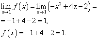Function limit and function value at a point x= 1 are equal. Therefore, the function is continuous at the point x = 1 .

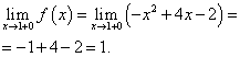
Dot x= 3 . Find the left-hand limit at this point:

Let's find the right-hand limit:

Function limit and function value at a point x= 3 must be found at the branch of the function that includes this point, that is, the second branch. We find them:

.

Function limit and function value at a point x= 3 are equal. Therefore, the function is continuous at the point x = 3 .

Main conclusion: this function is continuous at every boundary point.

Establish the continuity of a function at a point yourself, and then see the solution

A continuous change in a function can be defined as a change that is gradual, without jumps, in which a small change in the argument entails a small change in the function .

Let's illustrate this continuous change of function with an example.

Let a load hang on a thread above the table. Under the action of this load, the thread is stretched, so the distance l load from the point of suspension of the thread is a function of the mass of the load m, that is l = f(m) , m≥0 .

If we slightly change the mass of the load, then the distance l little change: little change m correspond to small changes l. However, if the mass of the load is close to the tensile strength of the thread, then a small increase in the mass of the load can cause the thread to break: the distance l will increase abruptly and become equal to the distance from the suspension point to the table surface. Function Graph l = f(m) shown in the figure. On the site, this graph is a continuous (solid) line, and at the point it is interrupted. The result is a graph consisting of two branches. At all points except , the function l = f(m) is continuous, and at a point it has a discontinuity.

The study of a function for continuity can be both an independent task and one of the stages of a complete study of the function and the construction of its graph.

Continuity of a function on an interval

Let the function y = f(x) defined in the interval ] a, b[ and is continuous at every point of this interval. Then it is called continuous in the interval ] a, b[ . The concept of continuity of a function on intervals of the form ]- ∞ is defined similarly, b[ , ]a, + ∞[ , ]- ∞, + ∞[ . Now let the function y = f(x) defined on the segment [ a, b] . The difference between an interval and a segment is that the boundary points of the interval are not included in the interval, but the boundary points of the segment are included in the segment. Here we should mention the so-called one-sided continuity: at the point a, staying on the interval [ a, b] , we can only approach from the right, and to the point b- only on the left. The function is called continuous on the segment [ a, b] , if it is continuous at all interior points of this segment, continuous on the right at the point a and left continuous at the point b.

Any of the elementary functions can serve as an example of a continuous function. Every elementary function is continuous on any segment on which it is defined. For example, the functions and are continuous on any interval [ a, b] , the function is continuous on the interval [ 0 , b] , the function is continuous on any segment that does not contain a point a = 2 .

Example 4 Investigate the function for continuity.

Solution. Let's check the first condition. The function is not defined at points - 3 and 3. At least one of the conditions for the continuity of the function on the entire number line is not satisfied. Therefore, this function is continuous on the intervals

Example 5 Determine at what value of the parameter a continuous throughout domains function

Solution.

Let's find the right-hand limit for:

.

It is obvious that the value at the point x= 2 must be equal ax :

a = 1,5 .

Example 6 Determine at what values ​​of the parameters a and b continuous throughout domains function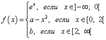

Solution.
Find the left-hand limit of the function at the point :

.

Therefore, the value at the point must be equal to 1:

Let's find the left-side function at the point :

Obviously, the value of the function at the point should be equal to:

Answer: the function is continuous over the entire domain of definition for a = 1; b = -3 .

Basic properties of continuous functions

Mathematics came to the concept of a continuous function by studying, first of all, various laws of motion. Space and time are endless and dependency like paths s from time t, expressed by law s = f(t) , gives an example of a continuous functions f(t) . The temperature of the heated water also changes continuously, it is also a continuous function of time: T = f(t) .

In mathematical analysis, some properties that continuous functions have have been proved. We present the most important of these properties.

1. If a function that is continuous on an interval takes on values ​​of different signs at the ends of the interval, then at some point of this segment it takes on a value equal to zero. More formally, this property is given in a theorem known as the first Bolzano-Cauchy theorem.

2. Function f(x) , continuous on the interval [ a, b] , takes all intermediate values ​​between the values ​​at the endpoints, that is, between f(a) and f(b) . More formally, this property is given in a theorem known as the second Bolzano-Cauchy theorem.