The second workshop is auxiliary elements. Absolute and relative coordinates
Martynyuk V.A.
Second Workshop - Supporting Elements 1
Coordinate systems in NX 7.5 1
Work coordinate system 2
Orientation RSK 3
When else do you need to remember about RSK 4
Basic coordinate systems 4
How to recover a lost base coordinate system 5
The concept of associativity 6
Auxiliary coordinate planes 8
Associated and fixed coordinate planes 9
Ways to build a coordinate plane 10
Auxiliary coordinate axes 11
Construction of perpendicular coordinate axes 12
Plotting points 14
The first way to plot points - precise input 14
Constructing a point with an offset relative to another point 15
Building a point on a face 15
Construction of a point on the auxiliary plane 16
Building point sets 17
Coordinate systems in Nx7.5
In the first workshop, we already mentioned that there are three coordinate systems in the NX7.5 system:
Working coordinate system - (RSK).
Basic coordinate systems(there may be several).
Absolute coordinate system which never changes its position. At the initial moment of working with a new project, all of the above coordinate systems coincide in place, and in orientation of the axes with the absolute coordinate system .

fig.1 fig.2
The very first thing you see on the screen, in the workspace, when you start a new project with template "Model"- this is:
Triad of vectors with a cube in the lower left corner of the screen (Fig. 1). It always shows the orientation of the axes absolute coordinate system in case of rotation of your model.
Two combined coordinate systems in the center (Fig. 2): RSK(colored arrows) and Base coordinate system(brown arrows), which coincide with the absolute coordinate system. On fig. 2 these two coordinate systems are combined. And herself absolute coordinate system considered invisible.
Working coordinate system
The working coordinate system (WCS) in the project is always the only one. But it can be arbitrarily moved in space. What for? The fact is that in NX7.5 there is a very important concept - working plane. it planeXOYworking coordinate system.
Why do we need the concept of a work plane? The fact is that in NX7.5, as in any other graphic system, there is flat construction apparatus. But if in other systems such a tool for flat constructions is only flatsketching , then in NX7.5 in addition to drawing flat sketches in the drop-down menu Paste \ Curves There is a wide range of tools available to help direct drawing of flat primitives without mentioning any sketches at all (Fig. 3).
But these are flat primitives. So they must be drawn in a plane! In what plane? Exactly in the working plane!
Thus, if you want to somehow arbitrarily orient a flat ellipse in space, you will have to first orient the RCS and its working plane accordingly. And only then, in this working plane, build, for example, an ellipse (Fig. 4).


Programming in absolute coordinates - G90. Programming in relative coordinates - G91. The G90 instruction will interpret the movements as absolute values with respect to the active zero point. The G91 instruction will interpret the moves as increments from previously reached positions. These instructions are modal.
Setting coordinate values - G92. The G92 instruction can be used in a block without axis (coordinate) information or with axis coordinate information. In the absence of axial information, all coordinate values are converted to the machine coordinate system; in this case, all compensations (corrections) and zero offset are removed. If axial information is available, the specified coordinate values become current. This instruction does not initiate any movements, it operates within one block.
N…G92 X0 Y0 /The current X and Y coordinates are set to zero. The current value of the Z coordinate remains unchanged.
N…G92 /Offsets and zero offsets are removed.
Plane selection - G17 (XY plane), G18 (XZ plane), G19 (YZ plane). The instructions define the choice of the work plane in the workpiece or program coordinate system. Operation of G02, G03, G05 instructions, polar coordinate programming, equidistant compensation are directly related to this selection.
Motion Paths (Interpolation Types)
Linear interpolation involves moving in a straight line in three-dimensional space. Before starting interpolation calculations, the TNC determines the length of the path based on the programmed coordinates. In the process of movement, the control of the contour feed is carried out so that its value does not exceed the allowable values. Movement along all coordinates must be completed simultaneously.
With circular interpolation, the movement is carried out along a circle in a given work plane. The parameters of the circle (for example, the coordinates of the end point and its center) are determined before the start of the movement, based on the programmed coordinates. In the process of movement, the control of the contour feed is carried out so that its value does not exceed the allowable values. Movement along all coordinates must be completed simultaneously.
Helical interpolation is a combination of circular and linear interpolation.
Linear interpolation at rapid traverse - G00, G200. During rapid motion, the programmed motion is interpolated and the movement to the end point is carried out in a straight line at the maximum feedrate. Feedrate and feedrate, for at least one axis, are maximum. The feedrate of the other axes is controlled so that the movement of all axes ends at the end point at the same time. While the G00 instruction is active, the movement decelerates to zero in every block. If it is not necessary to decelerate the feedrate to zero every block, then G200 is used instead of G00. The value of the maximum feedrate is not programmed, but is set by the so-called "machine parameters" in the memory of the CNC system. G00, G200 instructions are modal.
Linear interpolation with programmed feedrate - G01. Movement at the specified feedrate (in F word) towards the end point of the block is carried out in a straight line. All coordinate axes complete the movement at the same time. The feedrate at the end of the block is reduced to zero. The programmed feedrate is a contour feedrate, i.e. the feedrate values for each individual coordinate axis will be smaller. The feedrate value is usually limited by the setting of "machine parameters". Word combination variant with G01 instruction in the block: G01_X_Y_Z_F_.
Circular interpolation - G02, G03. The block is traversed in a circle at the contour speed specified in the active F word. Movement along all coordinate axes is completed simultaneously in the block. These instructions are modal. The feed drives specify a circular movement at the programmed feed in the selected interpolation plane; the G02 instruction specifies clockwise movement, while the G03 instruction specifies counterclockwise movement. When programming, a circle is defined using its radius or the coordinates of its center. An additional circle programming option is defined by the G05 instruction: circular interpolation with tangential path entry.
Programming a circle using a radius. The radius is always given in relative coordinates; in contrast to the end point of the arc, which can be specified in both relative and absolute coordinates. Using the position of the start and end points, as well as the value of the radius, the TNC first determines the coordinates of the circle. The result of the calculation can be the coordinates of two points ML, MR, located respectively to the left and to the right of the straight line connecting the start and end points.
The location of the center of the circle depends on the sign of the radius; with a positive radius, the center will be on the left, and with a negative radius, it will be on the right. The center location is also determined by the G02 and G03 instructions.
Variant of a word combination with a G03 instruction in a block: N_G17_G03_X_Y_R±_F_S_M. Here: instruction G17 means to select circular interpolation in the X/Y plane; the G03 instruction defines circular interpolation in the counterclockwise direction; X_Y_ are the coordinates of the end point of the circular arc; R is the radius of the circle.
Programming a circle using the coordinates of its center. The coordinate axes relative to which the position of the center is determined are parallel to the X, Y and Z axes, respectively, and the corresponding center coordinates are named I, J and K. The coordinates set the distances between the starting point of the circular arc and its center M in directions parallel to the axes. The sign is determined by the direction of the vector from A to M.
N… G90 G17 G02 X350 Y250 I200 J-50 F… S… M…
Full circle programming example: N… G17 G02 I… F… S… M…
Circular interpolation with tangential access to a circular path - G05. The CNC uses the G05 instruction to calculate such a circular section, which is reached tangentially from the previous block (with linear or circular interpolation). The parameters of the formed arc are determined automatically; those. only its end point is programmed, and the radius is not specified.
Helical interpolation - G202, G203. Helical interpolation consists of circular interpolation in the selected plane and linear interpolation for the remaining coordinate axes, up to a total of six rotary axes. The circular interpolation plane is defined by the G17, G18, G19 instructions. Clockwise circular movement is carried out according to the G202 instruction; counterclockwise circular motion - G203. Circle programming is possible both using the radius and using the coordinates of the center of the circle.
N… G17 G203 X… Y… Z… I… J… F… S… M…
Coordinates that indicate the location of a point, given the screen's coordinate system, are called absolute coordinates. For example, PSET(100,120) - means that a dot will appear on the screen 100 pixels to the right and 120 pixels below the upper left corner, i.e. screen origin.
The coordinates of the point that was last drawn are stored in the computer's memory. This point is called the last reference point (TLP). For example, if you specify only the coordinates of one point when drawing a line, then a segment from the TPS to the specified point will be drawn on the screen, which after that will become the TPS itself. Immediately after turning on graphics mode, the last link point is the point in the center of the screen.
In addition to absolute coordinates, QBASIC also uses relative coordinates. These coordinates show the amount of movement of the TPS. To draw a new point using relative coordinates, you need to use the STEP(X,Y) keyword, where X and Y are the offset of the coordinates relative to the TPS.
For example, PSET STEP(-5,10) - in this case, a point will appear, the position of which will be 5 points to the left and 10 points lower relative to the last link point. That is, if the point of the last link had coordinates, for example, (100,100), then a point with coordinates (95,110) will be obtained.
Drawing lines and rectangles.
LINE(X1,Y1)-(X2,Y2),C- draws a segment connecting the points (X1, Y1) and (X2, Y2) with color C.
For example, LINE(5,5)-(10,20),4
Result: 5 10
If you do not specify the first coordinate, then a segment will be drawn from the TPS to a point with coordinates (X2, Y2).
LINE(X1,Y1)-(X2,Y2), C, B- draws a rectangle outline with diagonal ends at points (X1, Y1) and (X2, Y2), C - color, B - rectangle marker.
For example, LINE(5,5)-(20,20), 5, V
Result: 5 20

If you specify BF instead of marker B, then a filled rectangle (block) will be drawn:
LINE(X1,Y1)-(X2,Y2),C, BF
For example, LINE(5,5)-(20,20),5, BF
 Result: 5 20
Drawing circles, ellipses and arcs.
CIRCLE(X,Y), R, C- draws a circle centered at the point (X, Y), radius R, color C.
For example, CIRCLE(50,50), 10, 7
Result:
 50
50
CIRCLE(X,Y), R, C, f1, f2- an arc of a circle, f1 and f2 arc angle values in radians from 0 to 6.2831, defining the beginning and end of the arc.
CIRCLE(X,Y), R, C, e- ellipse, centered at the point (X, Y), radius R, e - the ratio of the vertical axis to the horizontal.
For example, CIRCLE(50,50), 20, 15, 7, 1/2
Result: 30 50 70

If necessary, after the C parameter, you can specify the values of the ellipse arc angles f1 and f2.
PAINT(X,Y), C, K- paint with color C the figure drawn with color K, (X, Y) - a point lying inside the figure. If the outline color matches the fill color, then only one color is indicated: PAINT(X,Y), C
For example, you need to paint the circle CIRCLE(150,50), 40, 5 with color 4. To do this, you need to execute the PAINT(150,50), 4, 5 statement, because the center of the circle lies exactly inside the shape being filled, we used it as an interior point.
Problem solving.
Task 1.
Draw four points that lie on the same horizontal line at a distance of 20 pixels from each other. The last link point has coordinate (15, 20).
Solution: NOTES.
SCREEN 9: COLOR 5.15:REM graphic mode, background 5, color 15
CLS:REM screen cleaning
PSET(15,20) :REM draws a point at coordinates (15,20)
PSET STEP(20,0) :REM draws a point with an offset
PSET STEP(20,0) :REM relative to last by 20
PSET STEP(20,0) :REM pixels on the x-axis.
Result: 15 35 55 75

20. . . .
Task 2.
Draw three circles whose centers lie on the same horizontal line at a distance of 30 pixels from each other. The radii of the circles are 20, the center of the first circle coincides with the center of the screen.
Solution.
 SCREEN 9 120 150 180
CIRCLE STEP(0, 0), 20, 15 100
CIRCLE STEP(30, 0), 20, 15
CIRCLE STEP(30, 0), 20, 15
Task 2.
Construct a quadrilateral with vertices (10.15), (30.25), (30.5) and (20.0).
LINE (10,15)-(30,25), 5
LINE - (30, 5),5
LINE - (25,0), 5
LINE - (10,15), 5
RESULT: 5 10 20 25 30
 15
15
Write a program to draw an arbitrary picture.
Useful advice: Before you start writing a program, draw a picture on a piece of paper in a cage and arrange the desired coordinates. You will immediately see what numbers will be used as operands in your program.
Computer graphics
Tutorial
St. Petersburg
1.1. Fundamentals of working in the AutoCAD environment.. 4
1.2. Construction of a drawing using 3D technology. ten
1.3. Laboratory work №1. fifteen
1.4. Typical connections of parts. 19
1.5. Types of products and design documents. 27
1.6. Laboratory work №2. 32
2.1. Objects in 3ds Max. 39
2.2. Methods for transforming geometric objects. 45
2.3. Laboratory work №3. 48
2.4. loft modeling. fifty
2.5. Deformation of models built by the lofting method. 53
2.6. Laboratory work №4. 56
2.7. Mesh shells. 58
2.8. Editing meshes. 61
2.9. Laboratory work №5. 66
2.10. Sources of light. 67
2.11. Shooting Cameras.. 70
2.12. Materials.. 75
2.13. Laboratory work №6. 80
2.14. Animation. 82
2.15. Movement of objects along a given path. 86
2.16. Laboratory work №7. 88
3. Graphic programming. 90
3.1. Description of the DirectX Driver Set.. 90
3.2. Description of the OpenGL graphics system. 93
3.3. Fundamentals of OpenGL. 96
3.4. Drawing geometric objects. 102
3.5. Laboratory work №8. 107
References.. 110
AutoCAD is the world's most widely used system for computer-aided design and production of working design and project documentation. With its help, two-dimensional and three-dimensional projects of varying degrees of complexity are created in the field of architecture and construction, mechanical engineering, geodesy, etc. The AutoCAD data storage format is de facto recognized as the international standard for storing and transferring design documentation.
The main advantage of AutoCAD is the availability for creating powerful specialized calculation and graphics packages on its basis. Autodesk produces two main product lines designed for architects (Autodesk Architectural Desktop) and mechanical engineers (Autodesk Mechanical Desktop). All of these products use AutoCAD as their foundation.
The first version of MicroCAD (the prototype of AutoCAD) was released on August 25, 1982. This day is considered the release date of the first Autodesk product.
Fundamentals of working in the AutoCAD environment
Status bar
The status bar (Fig. 1.1) displays the current coordinates of the cursor and contains the buttons for turning on/off the drawing modes:
· SNAP - Snap Mode (Step-by-step binding) - inclusion and switching off of a step binding of the cursor;
· GRID - Grid Display - turn the grid on and off;
· ORTHO - Ortho Mode (Ortho Mode) - enable and disable the orthogonal mode;
· POLAR - Polar Tracking (Polar tracking) - turning on and off the polar tracking mode;
· OSNAP - Object Snap (Object snap) - enabling and disabling object snap modes;
· OTRACK - Object Snap Tracking (Tracking with object snap) - turning on and off the tracking mode with object snap;
· MODEL / PAPER - Model or Paper space (Model or paper space) - switching from model space to paper space;
· LWT - Show/Hide Lineweight (Display lines in accordance with weights) - turn on and off the mode of displaying lines in accordance with weights (thicknesses).
Rice. 1.1. Status bar
Using object snaps allows you to reduce the time of working on the drawing, since in some cases there is no need to manually enter coordinates, you just need to point the cursor at an already existing point belonging to some object.
Command line window
The “Command Line” window (Command line, Fig. 1.2) is usually located above the status bar and is used to enter commands and display prompts and messages from AutoCAD. On fig. 1.2 shows an example of creating a wedge (Wedge tool of the Solids toolbar) using the command line. It can be specified by specifying two opposite vertices of the base and height, or one vertex, length, height and width (for a wedge inscribed in a cube, the vertex and side value). When enumerating, the parameters are specified separated by commas. The separator between integer and fractional parts is a dot.

Rice. 1.2. Command line window
Coordinate systems
There are two coordinate systems in AutoCAD: the World Coordinate System (WCS) and the User Coordinate System (UCS). Only one coordinate system is active, which is usually called the current one. In it, the coordinates are determined by any available method.
The main difference between the world coordinate system and the user one is that there can be only one world coordinate system (for each model and paper space), and it is fixed. The use of a custom coordinate system has practically no restrictions. It can be located at any point in space at any angle to the world coordinate system. This is because it is easier to align a coordinate system with an existing geometry than it is to determine the exact placement of a point in 3D space.
To work with coordinate systems, use the "UCS" panel (Fig. 1.3). With its help, you can, for example, switch from the user coordinate system to the world one (the "World UCS" button) or align the coordinate system with an arbitrary object (the "Object UCS" button).
Rice. 1.3. UCS toolbar
Absolute and relative coordinates
In three-dimensional and two-dimensional space, both absolute coordinates (measured from the origin of coordinates) and relative (measured from the last specified point) are widely used. A sign of relative coordinates is the @ symbol before the coordinates of the specified point: “@<число 1>,<число 2>,<число 3>».
Typical views of objects
To represent the model in various views, the View toolbar (View, Fig. 1.4) is used. It allows you to present the model in both six standard views and four isometric views.

Rice. 1.4. View toolbar
To solve most problems in applied sciences, it is necessary to know the location of an object or point, which is determined using one of the accepted coordinate systems. In addition, there are elevation systems that also determine the altitude location of a point on
What are coordinates
Coordinates are numeric or literal values that can be used to determine the location of a point on the terrain. As a consequence, a coordinate system is a set of values of the same type that have the same principle for finding a point or object.
Finding the location of a point is required to solve many practical problems. In a science such as geodesy, determining the location of a point in a given space is the main goal, on the achievement of which all subsequent work is based.
Most coordinate systems, as a rule, define the location of a point on a plane limited by only two axes. In order to determine the position of a point in three-dimensional space, a system of heights is also used. With its help, you can find out the exact location of the desired object.
Briefly about coordinate systems used in geodesy
Coordinate systems determine the location of a point on a territory by giving it three values. The principles of their calculation are different for each coordinate system.

The main spatial coordinate systems used in geodesy:
- Geodetic.
- Geographic.
- Polar.
- Rectangular.
- Zonal Gauss-Kruger coordinates.
All systems have their own starting point, values for the location of the object and scope.
Geodetic coordinates
The main figure used to read geodetic coordinates is the earth's ellipsoid.
An ellipsoid is a three-dimensional compressed figure that best represents the figure of the globe. Due to the fact that the globe is a mathematically incorrect figure, it is the ellipsoid that is used instead to determine geodetic coordinates. This facilitates the implementation of many calculations to determine the position of the body on the surface.

Geodetic coordinates are defined by three values: geodetic latitude, longitude, and altitude.
- Geodetic latitude is an angle whose beginning lies on the plane of the equator, and the end lies at the perpendicular drawn to the desired point.
- Geodetic longitude is the angle that is measured from the zero meridian to the meridian on which the desired point is located.
- Geodetic height - the value of the normal drawn to the surface of the ellipsoid of the Earth's rotation from a given point.
Geographical coordinates
To solve high-precision problems of higher geodesy, it is necessary to distinguish between geodetic and geographical coordinates. In the system used in engineering geodesy, such differences, due to the small space covered by the work, as a rule, do not.
An ellipsoid is used as a reference plane to determine geodetic coordinates, and a geoid is used to determine geographical coordinates. The geoid is a mathematically incorrect figure, closer to the actual figure of the Earth. For its leveled surface, they take that which is continued under sea level in its calm state.

The geographic coordinate system used in geodesy describes the position of a point in space with three values. longitude coincides with the geodesic, since the reference point will also be called Greenwich. It passes through the observatory of the same name in the city of London. determined from the equator drawn on the surface of the geoid.
Height in the local coordinate system used in geodesy is measured from sea level in its calm state. On the territory of Russia and the countries of the former Union, the mark from which the heights are determined is the Kronstadt footstock. It is located at the level of the Baltic Sea.
Polar coordinates
The polar coordinate system used in geodesy has other nuances of the product of measurements. It is used in small areas of terrain to determine the relative location of a point. The reference point can be any object marked as a source. Thus, using polar coordinates, it is impossible to determine the unambiguous location of a point on the territory of the globe.

Polar coordinates are defined by two quantities: angle and distance. The angle is measured from the north direction of the meridian to a given point, determining its position in space. But one angle will not be enough, so a radius vector is introduced - the distance from the standing point to the desired object. With these two options, you can determine the location of the point in the local system.
As a rule, this coordinate system is used for engineering work carried out on a small area of area.
Rectangular coordinates
The rectangular coordinate system used in geodesy is also used in small areas of the terrain. The main element of the system is the coordinate axis from which the reference is made. The coordinates of a point are found as the length of perpendiculars drawn from the abscissa and ordinate axes to the desired point.

The north direction of the x-axis and the east of the y-axis are considered positive, and the south and west are negative. Depending on the signs and quarters, the location of a point in space is determined.
Gauss-Kruger coordinates
The Gauss-Kruger coordinate zonal system is similar to the rectangular one. The difference is that it can be applied to the entire territory of the globe, and not just to small areas.
The rectangular coordinates of the Gauss-Kruger zones, in fact, are the projection of the globe onto a plane. It arose for practical purposes to depict large areas of the Earth on paper. Transferring distortions are considered insignificant.
According to this system, the globe is divided by longitude into six-degree zones with the axial meridian in the middle. The equator is in the center along a horizontal line. As a result, there are 60 such zones.

Each of the sixty zones has its own system of rectangular coordinates, measured along the ordinate axis from X, and along the abscissa - from the area of the earth's equator Y. To unambiguously determine the location on the territory of the entire globe, the zone number is put in front of the X and Y values.
The values of the x-axis in Russia are usually positive, while the values of y can be negative. In order to avoid the minus sign in the values of the abscissa axis, the axial meridian of each zone is conditionally moved 500 meters to the west. Then all coordinates become positive.
The coordinate system was proposed by Gauss as possible and calculated mathematically by Krüger in the middle of the twentieth century. Since then, it has been used in geodesy as one of the main ones.
Height system
The systems of coordinates and heights used in geodesy are used to accurately determine the position of a point on the Earth. Absolute heights are measured from sea level or other surface taken as the original. In addition, there are relative heights. The latter are counted as an excess from the desired point to any other. It is convenient to use them for working in the local coordinate system in order to simplify the subsequent processing of the results.
Application of coordinate systems in geodesy
In addition to the above, there are other coordinate systems used in geodesy. Each of them has its own advantages and disadvantages. There are also their own areas of work for which this or that method of determining the location is relevant.
It is the purpose of the work that determines which coordinate systems used in geodesy are best used. For work in small areas, it is convenient to use rectangular and polar coordinate systems, and for solving large-scale problems, systems are needed that allow covering the entire territory of the earth's surface.