Determination of the location of equipotential and construction of lines of force of electric fields. Equipotential surfaces
For a more visual graphical representation of the fields, in addition to the lines of tension, use surfaces of equal potential or equipotential surfaces. As the name suggests, an equipotential surface is one in which all points have the same potential. If the potential is given as a function of x, y, z, then the equipotential surface equation is:
Field strength lines are perpendicular to equipotential surfaces.
Let's prove this statement.
Let the line and the line of force make up some angle (Fig. 1.5).
Let's move from point 1 to point 2 along the test charge line. In this case, the field forces do the work:
![]() . (1.5)
. (1.5)
 That is, the work of moving the test charge along the equipotential surface is zero. The same work can be defined in another way - as the product of the charge by the modulus of the field strength acting on the test charge, by the amount of displacement and by the cosine of the angle between the vector and the displacement vector, i.e. cosine of the angle (see fig. 1.5):
![]() .
.
The value of the work does not depend on the method of its calculation, according to (1.5) it is equal to zero. This implies that and, respectively, , which was to be proved.
An equipotential surface can be drawn through any point in the field. Therefore, an infinite number of such surfaces can be constructed. We agreed, however, to conduct the surfaces in such a way that the potential difference for two neighboring surfaces would be the same everywhere. Then, by the density of equipotential surfaces, one can judge the magnitude of the field strength. Indeed, the denser the equipotential surfaces are, the faster the potential changes when moving along the normal to the surface.
Figure 1.6,a shows the equipotential surfaces (more precisely, their intersection with the plane of the drawing) for the field of a point charge. In accordance with the nature of the change, the equipotential surfaces become denser when approaching the charge. Figure 1.6b shows the equipotential surfaces and lines of tension for the dipole field. From Fig. 1.6 it can be seen that with the simultaneous use of equipotential surfaces and lines of tension, the field picture is especially clear.

For a uniform field, equipotential surfaces obviously represent a system of equally spaced planes perpendicular to the direction of the field strength.
1.8. Relationship between field strength and potential
(potential gradient)
 Let there be an arbitrary electrostatic field. In this field, we draw two equipotential surfaces in such a way that they differ from one another by the potential by the value dφ(Fig. 1.7)
The tension vector is directed along the normal to the surface. The direction of the normal is the same as the direction of the x-axis. Axis x drawn from point 1 intersects the surface ![]() at point 2.
at point 2.
Line segment dx represents the shortest distance between points 1 and 2. The work done when the charge moves along this segment:
On the other hand, the same work can be written as:
Equating these two expressions, we get:
where the partial derivative symbol emphasizes that differentiation is carried out only with respect to x. Repeating similar reasoning for the axes y and z, we can find the vector :
![]() , (1.7)
, (1.7)
where are the unit vectors of the coordinate axes x, y, z.
The vector defined by expression (1.7) is called the scalar gradient φ . For it, along with the designation, the designation is also used. ("nabla") means a symbolic vector called the Hamilton operator
An electrostatic field can be characterized by a combination of force and equipotential lines.
force line - this is a line mentally drawn in the field, starting on a positively charged body and ending on a negatively charged body, drawn in such a way that the tangent to it at any point in the field gives the direction of tension at that point.
lines of force close on positive and negative charges and cannot close on themselves.
Under equipotential surface understand the set of field points that have the same potential ().
If the electrostatic field is cut by a secant plane, then traces of the intersection of the plane with equipotential surfaces will be visible in the section. These traces are called equipotential lines.
Equipotential lines are closed on themselves.
power lines and equipotential lines intersect at right angles.
R  Consider the equipotential surface:
 (since the points lie on an equipotential surface).


 - scalar product


The lines of the electrostatic field strength penetrate the equipotential surface at an angle of 90 0, then the angle between the vectors  is 90 degrees, and their dot product is 0.

Equipotential Line Equation
Consider the line of force:
H  the strength of the electrostatic field is directed tangentially to the field line (see the definition of the field line), the path element is also directed
  , so the angle between these two vectors is zero.
 or
or 
Field line equation
Gradient capacity
Gradient capacity is the rate of potential increase in the shortest direction between two points.
There is some potential difference between two points. If this difference is divided by the shortest distance between the points taken, then the resulting value will characterize the rate of potential change in the direction of the shortest distance between the points.
The potential gradient shows the direction of the greatest increase in the potential, is numerically equal to the intensity modulus and is negatively directed relative to it.
Two points are essential in the definition of a gradient:
The direction in which two nearby points are taken should be such that the rate of change is maximum.
The direction is that scalar function increases in this direction.


For a Cartesian coordinate system:


The rate of potential change in the direction of the X, Y, Z axis:
 ;
;  ;
;
Two vectors are equal only when their projections are equal to each other. The projection of the tension vector on the axis X is equal to the projection of the rate of potential change along the axis X taken with the opposite sign. Similarly for axes Y and Z.
 ;
;  ;
; .
.
In a cylindrical coordinate system, the expression for the potential gradient will have the following form.
Direction field line(tension lines) at each point coincides with the direction. Hence it follows that tension is equal to the potential difference U per unit length of the field line .
It is along the line of force that the maximum change in potential occurs. Therefore, it is always possible to determine between two points by measuring U between them, and the more accurate, the closer the points. In a uniform electric field, lines of force are straight. Therefore, it is easiest to define here:
A graphic representation of field lines and equipotential surfaces is shown in Figure 3.4.

When moving along this surface on d l potential will not change.
It follows that the projection of the vector to d l zero , that is Therefore, at each point it is directed along the normal to the equipotential surface.
You can draw as many equipotential surfaces as you like. By the density of equipotential surfaces, one can judge the value , this will be provided that the potential difference between two adjacent equipotential surfaces is equal to a constant value.
The formula expresses the relationship of potential with tension and allows you to known valuesφ find the field strength at each point. It is also possible to solve the inverse problem, i.e. by known values at each point of the field, find the potential difference between two arbitrary points of the field. To do this, we use the fact that the work done by the field forces on the charge q when moving it from point 1 to point 2 can be calculated as:
![]()
On the other hand, the work can be represented as:
![]() , then
, then ![]()
The integral can be taken along any line connecting point 1 and point 2, because the work of the field forces does not depend on the path. For a closed loop bypass, we get:
those. came to the well-known theorem on the circulation of the intensity vector: the circulation of the electrostatic field strength vector along any closed loop is equal to zero.
A field with this property is called potential.
From the vanishing of the circulation of the vector, it follows that the lines of the electrostatic field cannot be closed: they start on positive charges (sources) and on negative charges end (sinks) or go to infinity(Fig. 3.4).
This relation is true only for an electrostatic field. Subsequently, we will find out that the field of moving charges is not potential, and this relation is not satisfied for it.
Equipotential surface equipotential surface
a surface all of whose points have the same potential. The equipotential surface is orthogonal to the field lines. The surface of a conductor in electrostatics is an equipotential surface.
equipotential surfaceequipotential surface, a surface at all points of which the potential (cm. POTENTIAL (in physics)) electric field has the same value j= const. On a plane, these surfaces are equipotential field lines. Used to graphically display the potential distribution.
The equipotential surfaces are closed and do not intersect. The image of equipotential surfaces is carried out in such a way that the potential differences between adjacent equipotential surfaces are the same. In this case, in those areas where the lines of equipotential surfaces are denser, the field strength is greater.
Between any two points on the equipotential surface, the potential difference is zero. This means that the force vector at any point of the charge trajectory along the equipotential surface is perpendicular to the velocity vector. Therefore, the lines of tension (cm. ELECTRIC FIELD STRENGTH) electrostatic fields are perpendicular to the equipotential surface. In other words: the equipotential surface is orthogonal to the lines of force (cm. POWER LINES) field, and the electric field strength vector E is always perpendicular to the equipotential surfaces and is always directed in the direction of decreasing potential. The work of the forces of the electric field for any movement of the charge along the equipotential surface is zero, since?j = 0.
The equipotential surfaces of the field of a point electric charge are spheres, in the center of which the charge is located. The equipotential surfaces of a uniform electric field are planes perpendicular to the lines of tension. The surface of a conductor in an electrostatic field is an equipotential surface.
encyclopedic Dictionary. 2009 .
See what an "equipotential surface" is in other dictionaries:
A surface all of whose points have the same potential. The equipotential surface is orthogonal to the field lines. The surface of a conductor in electrostatics is an equipotential surface... Big Encyclopedic Dictionary
Surface, all points to the swarm have the same potential. For example, the surface of a conductor in electrostatics E. p. Physical encyclopedic Dictionary. Moscow: Soviet Encyclopedia. Editor-in-Chief A. M. Prokhorov. 1983... Physical Encyclopedia
equipotential surface- — [Ya.N. Luginsky, M.S. Fezi Zhilinskaya, Yu.S. Kabirov. English Russian Dictionary of Electrical Engineering and Power Engineering, Moscow, 1999] Topics in electrical engineering, basic concepts EN surface of equal potentialsequal energy surfaceequipotential ... ... Technical Translator's Handbook
The equipotential surfaces of an electric dipole (shown in dark are their sections by the plane of the figure; the color indicates the value of the potential in different points the highest values are purple and red, n ... Wikipedia
equipotential surface- vienodo potencialo paviršius statusas T sritis fizika atitikmenys: engl. equipotential surface vok. Äquipotentialfläche, f rus. equipotential surface, fpranc. surface depotential constant, f; surface d'égal potentiel, f; surface… … Fizikos terminų žodynas
A surface of equal potential, a surface all of whose points have the same Potential. For example, the surface of a conductor in electrostatics E. p. In a force field, the lines of force are normal (perpendicular) to E. p ... Big soviet encyclopedia
- (from lat. aequus equal and potential) geom. the place of points in the field, to the eye corresponds to the same value of the potential. E. p. are perpendicular to the lines of force. Equipotential is, for example, the surface of a conductor in an electrostatic ... ... Big encyclopedic polytechnic dictionary
For a visual representation of vector fields, a pattern of lines of force is used. The line of force is an imaginary mathematical
curve in space, the direction of the tangent to which in each
the point through which it passes coincides with the direction of the vector
fields at the same point(Fig. 1.17).
Rice. 1.17:
The condition of parallelism of the vector E → and the tangent can be written as equal to zero vector product E → and arc element d r → field line:
The equipotential is the surface which is a constant value of the electric potentialφ . In the field of a point charge, as shown in Fig. , spherical surfaces with centers at the location of the charge are equipotential; this can be seen from the equation ϕ = q ∕ r = const .
Analyzing the geometry of electric lines of force and equipotential surfaces, one can specify a series common properties geometry of the electrostatic field.
First, lines of force start at charges. They either go to infinity or end up on other charges, as in Fig. .
|
|

Secondly, in a potential field the lines of force cannot be closed. Otherwise, it would be possible to indicate such a closed loop that the work of the electric field when moving the charge along this loop is not equal to zero.
Thirdly, lines of force intersect any equipotential along the normal to it. Really, electric field everywhere is directed in the direction of the fastest decrease in the potential, and on the equipotential surface the potential is constant by definition (Fig. ). 
Rice. 1.20 :
And finally, the lines of force do not intersect anywhere except for the points where E → = 0 . The intersection of field lines means that the field at the intersection point is an ambiguous function of coordinates, and the vector E → has no definite direction. The only vector that has this property is the null vector. The structure of the electric field near the zero point will be analyzed in problems to ?? .
The method of lines of force, of course, is applicable to the graphical representation of any vector fields. So, in the chapter we will meet the concept of magnetic lines of force. However, the geometry magnetic field completely different from the geometry of the electric field.

Rice. 1.21:
The concept of lines of force is closely related to the concept of a force tube. Let us take any arbitrary closed loop L and draw an electric line of force through each point of it (Fig. ). These lines form the force tube. Consider an arbitrary section of the tube by the surface S . We draw a positive normal in the same direction as the lines of force are directed. Let N be the flow of the vector E → through the section S . It is easy to see that if there are no electric charges inside the tube, then the flux N remains the same along the entire length of the tube. To prove it, we need to take another cross section S ′. According to the Gauss theorem, the flow of the electric field through a closed surface limited by the side surface of the tube and sections S , S ′ is equal to zero, since there are no electric charges inside the force tube. flow through side surface is zero, since the vector E → touches this surface. Therefore, the flow through the section S ′ is numerically equal to N , but opposite in sign. The outer normal to the closed surface on this section is directed oppositely n → . If we direct the normal in the same direction, then the flows through the sections S and S ′ will coincide both in magnitude and in sign. In particular, if the tube is infinitely thin and the sections S and S′ are normal to it, then
E S = E′ S′ .
It turns out a complete analogy with the flow of an incompressible fluid. Where the tube is thinner, the field E → is stronger. In those places where it is wider, the field E → stronger. Therefore, the strength of the electric field can be judged from the density of the lines of force.
Before the invention of computers, for the experimental reproduction of field lines, a glass vessel with a flat bottom was taken and a non-conductive liquid, such as castor oil or glycerin, was poured into it. Powdered crystals of gypsum, asbestos or any other oblong particles were evenly mixed into the liquid. Metal electrodes were immersed in the liquid. When connected to sources of electricity, the electrodes excited an electric field. In this field, the particles are electrified and, being attracted to each other by oppositely electrified ends, are arranged in the form of chains along the lines of force. The picture of field lines is distorted by fluid flows caused by forces acting on it in an inhomogeneous electric field.
To Be Done Yet
Rice. 1.22:
The best results are obtained by the method used by Robert W. Pohl (1884-1976). Steel electrodes are glued onto a glass plate, between which an electrical voltage is created. Then, elongated particles, for example, gypsum crystals, are poured onto the plate, lightly tapping on it. They are located along it along the lines of force. On fig. ?? the picture of lines of force obtained in this way between two oppositely charged circles of frame is depicted.
▸ Task 9.1
Write the equation of field lines in arbitrary orthogonal coordinates.
▸ Task 9.2
Write down the equation of force lines in spherical coordinates.