Variance formula for grouped data. Variance and standard deviation
Dispersion is a measure of dispersion that describes the relative deviation between data values and the mean. It is the most commonly used measure of dispersion in statistics, calculated by summing, squared, the deviation of each data value from the mean. The formula for calculating the variance is shown below:
![]()
s 2 - sample variance;
x cf is the mean value of the sample;
n — sample size (number of data values),
(x i – x cf) is the deviation from the mean value for each value of the data set.
To better understand the formula, let's look at an example. I don't really like cooking, so I rarely do it. However, in order not to die of hunger, from time to time I have to go to the stove to implement the plan to saturate my body with proteins, fats and carbohydrates. The data set below shows how many times Renat cooks food each month:
The first step in calculating the variance is to determine the sample mean, which in our example is 7.8 times a month. The remaining calculations can be facilitated with the help of the following table.

The final phase of calculating the variance looks like this:
![]()
For those who like to do all the calculations in one go, the equation will look like this:
Using the raw count method (cooking example)
There is more effective method calculating the variance, known as the "raw counting" method. Although at first glance the equation may seem quite cumbersome, in fact it is not so scary. You can verify this, and then decide which method you like best.

is the sum of each data value after squaring,
is the square of the sum of all data values.
Don't lose your mind right now. Let's put it all in the form of a table, and then you will see that there are fewer calculations here than in the previous example.


As you can see, the result is the same as when using the previous method. Advantages this method become apparent as the sample size (n) grows.
Calculating variance in Excel
As you probably already guessed, Excel has a formula that allows you to calculate the variance. Moreover, starting from Excel 2010, you can find 4 varieties of the dispersion formula:
1) VAR.V - Returns the variance of the sample. Boolean values and text are ignored.
2) VAR.G - Returns the population variance. Boolean values and text are ignored.
3) VASP - Returns the sample variance, taking into account boolean and text values.
4) VARP - Returns the variance of the population, taking into account logical and text values.
First, let's look at the difference between a sample and a population. The purpose of descriptive statistics is to summarize or display data in such a way as to quickly get a big picture, so to speak, an overview. Statistical inference allows you to make inferences about a population based on a sample of data from this population. The population represents all possible outcomes or measurements that are of interest to us. A sample is a subset of a population.
For example, we are interested in the totality of a group of students of one of Russian universities and we need to determine the average score of the group. We can calculate the average performance of students, and then the resulting figure will be a parameter, since the whole population will be involved in our calculations. However, if we want to calculate the GPA of all students in our country, then this group will be our sample.
The difference in the formula for calculating the variance between the sample and the population is in the denominator. Where for the sample it will be equal to (n-1), and for the general population only n.
Now let's deal with the functions of calculating the variance with endings BUT, in the description of which it is said that the calculation takes into account text and logical values. In this case, when calculating the variance of a certain data array, where there are not numerical values, Excel will interpret text and false booleans as 0, and true booleans as 1.
So, if you have an array of data, it will not be difficult to calculate its variance using one of the Excel functions listed above.

Dispersionrandom variable- a measure of the dispersion of a given random variable, that is, her deviations from mathematical expectation. In statistics, the notation (sigma squared) is often used to denote variance. The square root of the variance is called standard deviation or standard spread. The standard deviation is measured in the same units as the random value, and the variance is measured in the squares of that unit.
Although it is very convenient to use only one value (such as mean or mode and median) to estimate the entire sample, this approach can easily lead to incorrect conclusions. The reason for this situation lies not in the value itself, but in the fact that one value does not in any way reflect the spread of data values.
For example, in the sample:
the average is 5.
However, there is no element in the sample itself with a value of 5. You may need to know how close each element of the sample is to its mean value. Or, in other words, you need to know the variance of the values. Knowing the extent to which the data has changed, you can better interpret mean, median and fashion. The degree of change in sample values is determined by calculating their variance and standard deviation.
The variance and the square root of the variance, called the standard deviation, characterize the mean deviation from the sample mean. Among these two quantities, the most important is standard deviation. This value can be represented as the average distance at which the elements are from the middle element of the sample.
Dispersion is difficult to interpret meaningfully. However, the square root of this value is the standard deviation and lends itself well to interpretation.
The standard deviation is calculated by first determining the variance and then calculating square root from dispersion.
For example, for the data array shown in the figure, the following values will be obtained:

Picture 1
Here, the mean of the squared differences is 717.43. To get the standard deviation, it remains only to take the square root of this number.
The result will be approximately 26.78.
It should be remembered that the standard deviation is interpreted as the average distance at which the elements are from the sample mean.
The standard deviation shows how well the mean describes the entire sample.
Let's say you are the manager production department PC assembly. The quarterly report says that the output for the last quarter was 2500 PCs. Is it bad or good? You asked (or there is already this column in the report) to display the standard deviation for this data in the report. The standard deviation figure, for example, is 2000. It becomes clear to you, as the head of the department, that the production line requires better management(too large deviations in the number of assembled PCs).
Recall that when the standard deviation is large, the data is widely scattered around the mean, and when the standard deviation is small, it clusters close to the mean.
Four statistical functions VARP(), VARP(), STDEV() and STDEV() are designed to calculate the variance and standard deviation of numbers in a range of cells. Before you can calculate the variance and standard deviation of a data set, you need to determine whether the data represents the population or a sample of the population. In the case of a sample from the general population, the VARP() and STDEV() functions should be used, and in the case of the general population, the VARP() and STDEV() functions should be used:
| Population | Function |
 | VARP() |
 | STDLONG() |
| Sample | |
 | VARI() |
 | STDEV() |
The variance (as well as the standard deviation), as we noted, indicates the extent to which the values included in the data set are scattered around the arithmetic mean.
A small value of the variance or standard deviation indicates that all data are centered around the arithmetic mean, and great importance these values - that the data are scattered over a wide range of values.
The variance is rather difficult to interpret meaningfully (what does a small value mean, a large value?). Performance Tasks 3 will allow you to visually, on a graph, show the meaning of the variance for a data set.
Tasks
· Exercise 1.
· 2.1. Give the concepts: variance and standard deviation; their symbolic designation in statistical data processing.
· 2.2. Draw up a worksheet in accordance with Figure 1 and make the necessary calculations.
· 2.3. Give the basic formulas used in the calculations
· 2.4. Explain all notation ( , , )
· 2.5. explain practical value the concepts of variance and standard deviation.
Task 2.
1.1. Give the concepts: general population and sample; mathematical expectation and arithmetic mean of their symbolic designation in statistical data processing.
1.2. In accordance with Figure 2, draw up a worksheet and make calculations.
1.3. Give the basic formulas used in the calculations (for the general population and sample).

Figure 2
1.4. Explain why it is possible to obtain such values of arithmetic means in samples as 46.43 and 48.78 (see file Appendix). To conclude.
Task 3.
There are two samples with a different set of data, but the average for them will be the same:

Figure 3
3.1. Draw up a worksheet in accordance with Figure 3 and make the necessary calculations.
3.2. Give the basic calculation formulas.
3.3. Build graphs in accordance with figures 4, 5.
3.4. Explain the resulting dependencies.
3.5. Perform similar calculations for these two samples.
Initial sample 11119999
Select the values of the second sample so that the arithmetic mean for the second sample is the same, for example:

Pick the values for the second sample yourself. Arrange calculations and plotting like figures 3, 4, 5. Show the main formulas that were used in the calculations.
Draw the appropriate conclusions.
All tasks should be presented in the form of a report with all the necessary figures, graphs, formulas and brief explanations.
Note: the construction of graphs must be explained with figures and brief explanations.
However, this characteristic alone is not yet sufficient for the study of a random variable. Imagine two shooters who are shooting at a target. One shoots accurately and hits close to the center, and the other ... just having fun and not even aiming. But what's funny is that average the result will be exactly the same as the first shooter! This situation is conditionally illustrated by the following random variables:
The "sniper" mathematical expectation is equal to , however, " interesting personality»: - it is also zero!
Thus, there is a need to quantify how far scattered bullets (values of a random variable) relative to the center of the target (expectation). well and scattering translated from Latin only as dispersion .
Let's see how this numerical characteristic is determined in one of the examples of the 1st part of the lesson: 
There we found a disappointing mathematical expectation of this game, and now we have to calculate its variance, which denoted through .
Let's find out how far the wins/losses are "scattered" relative to the average value. Obviously, for this we need to calculate differences between values of a random variable and her mathematical expectation:
–5 – (–0,5) = –4,5
2,5 – (–0,5) = 3
10 – (–0,5) = 10,5
Now it seems to be necessary to sum up the results, but this way is not good - for the reason that the oscillations to the left will cancel each other out with the oscillations to the right. So, for example, the "amateur" shooter (example above) the differences will be ![]() , and when added they will give zero, so we will not get any estimate of the scattering of his shooting.
, and when added they will give zero, so we will not get any estimate of the scattering of his shooting.
To get around this annoyance, consider modules differences, but for technical reasons, the approach has taken root when they are squared. It is more convenient to arrange the solution in a table: 
And here it begs to calculate weighted average the value of the squared deviations. What is it? It's theirs expected value, which is the measure of scattering:
![]() – definition dispersion. It is immediately clear from the definition that variance cannot be negative- take note for practice!
– definition dispersion. It is immediately clear from the definition that variance cannot be negative- take note for practice!
Let's remember how to find the expectation. Multiply the squared differences by the corresponding probabilities (Table continuation):
- figuratively speaking, this is "traction force",
and summarize the results:
Don't you think that against the background of winnings, the result turned out to be too big? That's right - we were squaring, and in order to return to the dimension of our game, we need to take the square root. This value is called standard deviation
and is denoted by the Greek letter "sigma":
Sometimes this meaning is called standard deviation .
What is its meaning? If we deviate from the mathematical expectation to the left and to the right by the standard deviation: ![]()
– then the most probable values of the random variable will be “concentrated” on this interval. What we are actually seeing:
However, it so happened that in the analysis of scattering almost always operate with the concept of dispersion. Let's see what it means in relation to games. If in the case of shooters we are talking about the "accuracy" of hits relative to the center of the target, then here the dispersion characterizes two things:
First, it is obvious that as the rates increase, the variance also increases. So, for example, if we increase by 10 times, then the mathematical expectation will increase by 10 times, and the variance will increase by 100 times (as soon as it is a quadratic value). But note that the rules of the game have not changed! Only the rates have changed, roughly speaking, we used to bet 10 rubles, now 100.
Second, more interesting point is that the variance characterizes the style of the game. Mentally fix the game rates at some certain level, and see what's what here:
A low variance game is a cautious game. The player tends to choose the most reliable schemes, where he does not lose/win too much at one time. For example, the red/black system in roulette (see Example 4 of the article random variables) .
High variance game. She is often called dispersion game. Is it adventurous or aggressive style games where the player chooses "adrenaline" schemes. Let's at least remember "Martingale", in which the sums at stake are orders of magnitude greater than the “quiet” game of the previous paragraph.
The situation in poker is indicative: there are so-called tight players who tend to be cautious and "shake" over their game means (bankroll). Not surprisingly, their bankroll does not fluctuate much (low variance). Conversely, if a player has high variance, then it is the aggressor. He often takes risks, makes large bets and can both break a huge bank and go to pieces.
The same thing happens in Forex, and so on - there are a lot of examples.
Moreover, in all cases it does not matter whether the game is for a penny or for thousands of dollars. Every level has its low and high variance players. Well, for the average win, as we remember, "responsible" expected value.
You probably noticed that finding the variance is a long and painstaking process. But mathematics is generous:
Formula for finding the variance
This formula is derived directly from the definition of variance, and we immediately put it into circulation. I will copy the plate with our game from above: 
and the found expectation .
We calculate the variance in the second way. First, let's find the mathematical expectation - the square of the random variable . By definition of mathematical expectation:
In this case:
Thus, according to the formula:
As they say, feel the difference. And in practice, of course, it is better to apply the formula (unless the condition requires otherwise).
We master the technique of solving and designing:
Example 6

Find its mathematical expectation, variance and standard deviation.
This task is found everywhere, and, as a rule, goes without a meaningful meaning.
You can imagine several light bulbs with numbers that light up in a madhouse with certain probabilities :)
Solution: It is convenient to summarize the main calculations in a table. First, we write the initial data in the top two lines. Then we calculate the products, then and finally the sums in the right column: 
Actually, almost everything is ready. In the third line, a ready-made mathematical expectation was drawn: ![]() .
.
The dispersion is calculated by the formula:
And finally, the standard deviation:
- personally, I usually round to 2 decimal places.
All calculations can be carried out on a calculator, and even better - in Excel:
It's hard to go wrong here :)
Answer:
Those who wish can simplify their lives even more and take advantage of my calculator (demo), which not only instantly solves this problem, but also builds thematic graphics (come soon). The program can download in the library– if you have downloaded at least one educational material or get another way. Thanks for supporting the project!
A couple of tasks for independent decision:
Example 7
Calculate the variance of the random variable of the previous example by definition.
And a similar example:
Example 8
A discrete random variable is given by its own distribution law:

Yes, the values of the random variable can be quite large (example from real work) , and here, if possible, use Excel. As, by the way, in Example 7 - it is faster, more reliable and more pleasant.
Solutions and answers at the bottom of the page.
At the end of the 2nd part of the lesson, we will analyze one more typical task, one might even say, a small rebus:
Example 9
A discrete random variable can take only two values: and , and . The probability, mathematical expectation and variance are known.
Solution: Let's start with an unknown probability. Since a random variable can take only two values, then the sum of the probabilities of the corresponding events:
and since , then .
It remains to find ..., easy to say :) But oh well, it started. By definition of mathematical expectation: ![]() - substitute the known values:
- substitute the known values:
![]() - and nothing more can be squeezed out of this equation, except that you can rewrite it in the usual direction:
- and nothing more can be squeezed out of this equation, except that you can rewrite it in the usual direction: ![]()

or: ![]()
About further actions, I think you can guess. Let's create and solve the system: 
Decimals- this, of course, is a complete disgrace; multiply both equations by 10: 
and divide by 2: 
That's much better. From the 1st equation we express: ![]() (this is the easier way)- substitute in the 2nd equation:
(this is the easier way)- substitute in the 2nd equation:
![]()
We are building squared and make simplifications: 
We multiply by: 
As a result, quadratic equation, find its discriminant:
- perfect!
and we get two solutions:
1) if ![]() , then
, then ![]() ;
;
2) if ![]() , then .
, then .
The first pair of values satisfies the condition. With a high probability, everything is correct, but, nevertheless, we write down the distribution law: 
and perform a check, namely, find the expectation:
Often in statistics, when analyzing a phenomenon or process, it is necessary to take into account not only information about the average levels of the studied indicators, but also scatter or variation in the values of individual units , which is important characteristic studied population.
Stock prices, volumes of supply and demand, interest rates in different periods time and in different places.
The main indicators characterizing the variation , are the range, variance, standard deviation and coefficient of variation.
Span variation is the difference between the maximum and minimum values of the attribute: R = Xmax – Xmin. The disadvantage of this indicator is that it evaluates only the boundaries of the trait variation and does not reflect its fluctuation within these boundaries.
Dispersion devoid of this shortcoming. It is calculated as the average square of deviations of the attribute values from their average value:
Simplified way to calculate variance is carried out using the following formulas (simple and weighted):
Examples of the application of these formulas are presented in tasks 1 and 2.
A widely used indicator in practice is standard deviation :
The standard deviation is defined as the square root of the variance and has the same dimension as the trait under study.
The considered indicators make it possible to obtain the absolute value of the variation, i.e. evaluate it in units of measure of the trait under study. Unlike them, the coefficient of variation measures fluctuation in relative terms - relative to the average level, which in many cases is preferable.
Formula for calculating the coefficient of variation.
Examples of solving problems on the topic "Indicators of variation in statistics"
Task 1 . When studying the influence of advertising on the size of the average monthly deposit in the banks of the region, 2 banks were examined. The following results are obtained:
Define:
1) for each bank: a) average monthly deposit; b) dispersion of the contribution;
2) the average monthly deposit for two banks together;
3) Dispersion of the deposit for 2 banks, depending on advertising;
4) Dispersion of the deposit for 2 banks, depending on all factors except advertising;
5) Total variance using the addition rule;
6) Coefficient of determination;
7) Correlation relation.
Solution
1) Let's make a calculation table for a bank with advertising . To determine the average monthly deposit, we find the midpoints of the intervals. In this case, the value of the open interval (the first one) is conditionally equated to the value of the interval adjacent to it (the second one).
We find the average size of the contribution using the weighted arithmetic mean formula:
29,000/50 = 580 rubles
The dispersion of the contribution is found by the formula:
23 400/50 = 468
We will perform similar actions for a bank without ads :
2) Find the average deposit for two banks together. Xav \u003d (580 × 50 + 542.8 × 50) / 100 \u003d 561.4 rubles.
3) The variance of the deposit, for two banks, depending on advertising, we will find by the formula: σ 2 =pq (formula of the variance of an alternative sign). Here p=0.5 is the proportion of factors that depend on advertising; q=1-0.5, then σ 2 =0.5*0.5=0.25.
4) Since the share of other factors is 0.5, then the variance of the deposit for two banks, which depends on all factors except advertising, is also 0.25.
5) Determine the total variance using the addition rule.
= (468*50+636,16*50)/100=552,08
= [(580-561,4)250+(542,8-561,4)250] / 100= 34 596/ 100=345,96
σ 2 \u003d σ 2 fact + σ 2 rest \u003d 552.08 + 345.96 \u003d 898.04
6) Coefficient of determination η 2 = σ 2 fact / σ 2 = 345.96/898.04 = 0.39 = 39% - the size of the contribution depends on advertising by 39%.
7) Empirical correlation ratio η = √η 2 = √0.39 = 0.62 - the relationship is quite close.
Task 2 . There is a grouping of enterprises according to the value of marketable products:
Determine: 1) the dispersion of the value of marketable products; 2) standard deviation; 3) coefficient of variation.
Solution
1) By condition, an interval distribution series is presented. It must be expressed discretely, that is, find the middle of the interval (x "). In groups of closed intervals, we find the middle by a simple arithmetic mean. In groups with an upper limit, as the difference between this upper limit and half the size of the interval following it (200-(400 -200):2=100).
In groups with a lower limit - the sum of this lower limit and half the size of the previous interval (800+(800-600):2=900).
The calculation of the average value of marketable products is done according to the formula:
Хср = k×((Σ((x"-a):k)×f):Σf)+a. Here a=500 is the size of the variant at the highest frequency, k=600-400=200 is the size of the interval at the highest frequency Let's put the result in a table:
So, the average value of marketable output for the period under study as a whole is Xav = (-5:37) × 200 + 500 = 472.97 thousand rubles.
2) We find the dispersion using the following formula:
σ 2 \u003d (33/37) * 2002-(472.97-500) 2 \u003d 35,675.67-730.62 \u003d 34,945.05
3) standard deviation: σ = ±√σ 2 = ±√34 945.05 ≈ ±186.94 thousand rubles.
4) coefficient of variation: V \u003d (σ / Xav) * 100 \u003d (186.94 / 472.97) * 100 \u003d 39.52%
Variation range (or range of variation) - is the difference between the maximum and minimum values of the feature:
In our example, the range of variation in shift output of workers is: in the first brigade R=105-95=10 children, in the second brigade R=125-75=50 children. (5 times more). This suggests that the output of the 1st brigade is more “stable”, but the second brigade has more reserves for the growth of output, because. if all workers reach the maximum output for this brigade, it can produce 3 * 125 = 375 parts, and in the 1st brigade only 105 * 3 = 315 parts.
If the extreme values of the attribute are not typical for the population, then quartile or decile ranges are used. The quartile range RQ= Q3-Q1 covers 50% of the population, the first decile range RD1 = D9-D1 covers 80% of the data, the second decile range RD2= D8-D2 covers 60%.
The disadvantage of the variation range indicator is, but that its value does not reflect all the fluctuations of the trait.
The simplest generalizing indicator that reflects all the fluctuations of a trait is mean linear deviation, which is the arithmetic mean of the absolute deviations of individual options from their average value:
,
for grouped data ![]() ,
,
where хi is the value of the attribute in a discrete series or the middle of the interval in the interval distribution.
In the above formulas, the differences in the numerator are taken modulo, otherwise, according to the property of the arithmetic mean, the numerator will always be equal to zero. Therefore, the average linear deviation is rarely used in statistical practice, only in those cases where summing the indicators without taking into account the sign makes economic sense. With its help, for example, the composition of employees, the profitability of production, and foreign trade turnover are analyzed.
Feature variance is the average square of the deviations of the variant from their average value:
simple variance ![]() ,
,
weighted variance  .
.
The formula for calculating the variance can be simplified:
Thus, the variance is equal to the difference between the mean of the squares of the variant and the square of the mean of the variant of the population:  .
.
However, due to the summation of the squared deviations, the variance gives a distorted idea of the deviations, so the average is calculated from it. standard deviation, which shows how much the specific variants of the attribute deviate on average from their average value. Calculated by taking the square root of the variance:
for ungrouped data  ,
,
for the variation series 
How less value dispersion and standard deviation, the more homogeneous the population, the more reliable (typical) the average value will be.
Linear Mean and Mean standard deviation- named numbers, that is, they are expressed in units of measurement of the attribute, are identical in content and close in meaning.
It is recommended to calculate the absolute indicators of variation using tables.
Table 3 - Calculation of the characteristics of variation (on the example of the period of data on the shift output of the work teams)
Number of workers |
The middle of the interval |
Estimated values |
|||||
Total: |
|||||||
Average shift output of workers: ![]()
Average linear deviation: ![]()
Output dispersion: 
The standard deviation of the output of individual workers from the average output:
.
1 Calculation of dispersion by the method of moments
The calculation of variances is associated with cumbersome calculations (especially if the average value is expressed a large number with multiple decimal places). Calculations can be simplified by using a simplified formula and dispersion properties.
The dispersion has the following properties:
- if all the values of the attribute are reduced or increased by the same value A, then the variance will not decrease from this:
 ,
,
 , then or
Using the properties of the variance and first reducing all the variants of the population by the value A, and then dividing by the value of the interval h, we obtain a formula for calculating the variance in variational series with equal intervals way of moments: ,
,
where is the dispersion calculated by the method of moments;
h is the value of the interval of the variation series;
– new (transformed) variant values;
A is a constant value, which is used as the middle of the interval with the highest frequency; or the variant with the highest frequency;  is the square of the moment of the first order;
is a moment of the second order.
Let's calculate the variance by the method of moments based on the data on the shift output of the working team.
Table 4 - Calculation of dispersion by the method of moments
Groups of production workers, pcs. |
Number of workers |
The middle of the interval |
Estimated values |
||
Calculation procedure:


- calculate the variance:
2 Calculation of the variance of an alternative feature
Among the signs studied by statistics, there are those that have only two mutually exclusive meanings. These are alternative signs. They are given two quantitative values, respectively: options 1 and 0. The frequency of options 1, which is denoted by p, is the proportion of units that have this feature. The difference 1-p=q is the frequency of options 0. Thus,
xi |
|
Arithmetic mean of alternative feature ![]() , since p+q=1.
, since p+q=1.
Feature variance
, because 1-p=q
Thus, the variance of an alternative attribute is equal to the product of the proportion of units that have this attribute and the proportion of units that do not have this attribute.
If the values 1 and 0 are equally frequent, i.e. p=q, the variance reaches its maximum pq=0.25.
Variance variable is used in sample surveys, for example, product quality.
3 Intergroup dispersion. Variance addition rule
Dispersion, unlike other characteristics of variation, is an additive quantity. That is, in the aggregate, which is divided into groups according to the factor criterion X , resultant variance y can be decomposed into variance within each group (within group) and variance between groups (between group). Then, along with the study of the variation of the trait throughout the population as a whole, it becomes possible to study the variation in each group, as well as between these groups.
Total variance measures the variation of a trait at over the entire population under the influence of all the factors that caused this variation (deviations). It is equal to the mean square of the deviations of the individual values of the feature at of the overall mean and can be calculated as simple or weighted variance.
Intergroup variance characterizes the variation of the effective feature at, caused by the influence of the sign-factor X underlying the grouping. It characterizes the variation of the group means and is equal to the mean square of the deviations of the group means from the total mean:  ,
,
where is the arithmetic mean of the i-th group;
– number of units in the i-th group (frequency of the i-th group);
is the total mean of the population.
Intragroup variance reflects random variation, i.e., that part of the variation that is caused by the influence of unaccounted for factors and does not depend on the attribute-factor underlying the grouping. It characterizes the variation individual values relative to group means, equal to the mean square of the deviations of individual values of the attribute at within a group from the arithmetic mean of this group (group mean) and is calculated as a simple or weighted variance for each group: ![]() or
or ![]() ,
,
where is the number of units in the group.
Based on the intra-group variances for each group, it is possible to determine the overall average of the within-group variances:
.
The relationship between the three variances is called variance addition rules, according to which the total variance is equal to the sum of the intergroup variance and the average of the intragroup variances:
Example. When studying the influence tariff category(qualification) of workers on the level of productivity of their labor, the following data were obtained.
Table 5 - Distribution of workers by average hourly output.
№ p/p |
Workers of the 4th category |
Workers of the 5th category |
|||||
Working out |
Working out |
||||||
1 |
7 |
7-10=-3 |
9 |
1 |
14 |
14-15=-1 |
1 |
In this example, the workers are divided into two groups according to the factor X- qualifications, which are characterized by their rank. The effective trait - production - varies both under its influence (intergroup variation) and due to other random factors (intragroup variation). The challenge is to measure these variations using three variances: total, between-group, and within-group. The empirical coefficient of determination shows the proportion of the variation of the resulting feature at under the influence of a factor sign X. The rest of the total variation at caused by changes in other factors.
In the example, the empirical coefficient of determination is: ![]() or 66.7%,
or 66.7%,
This means that 66.7% of the variation in labor productivity of workers is due to differences in qualifications, and 33.3% is due to the influence of other factors.
Empirical correlation relation shows the tightness of the relationship between the grouping and effective features. It is calculated as the square root of the empirical coefficient of determination:
The empirical correlation ratio , as well as , can take values from 0 to 1.
If there is no connection, then =0. In this case, =0, that is, the group means are equal to each other and there is no intergroup variation. This means that the grouping sign - the factor does not affect the formation of the general variation.
If the relationship is functional, then =1. In this case, the variance of the group means is equal to the total variance (), i.e., there is no intragroup variation. This means that the grouping feature completely determines the variation of the resulting feature being studied.
The closer the value of the correlation relation is to one, the closer, closer to the functional dependence, the relationship between the features.
For a qualitative assessment of the closeness of the connection between the signs, the Chaddock relations are used.
In the example ![]() , which indicates a close relationship between the productivity of workers and their qualifications.
, which indicates a close relationship between the productivity of workers and their qualifications.